[MATLAB 영상처리 기초 6] 선형 공간 필터링 - Average, Laplacian, Sobel filters

 

 

 

선형 공간 필터링(linear spatial filtering) 소개 동영상

 

 

 

 

 

Cells from cervical cancer - National Cancer Institute (출처2)

 

 

 

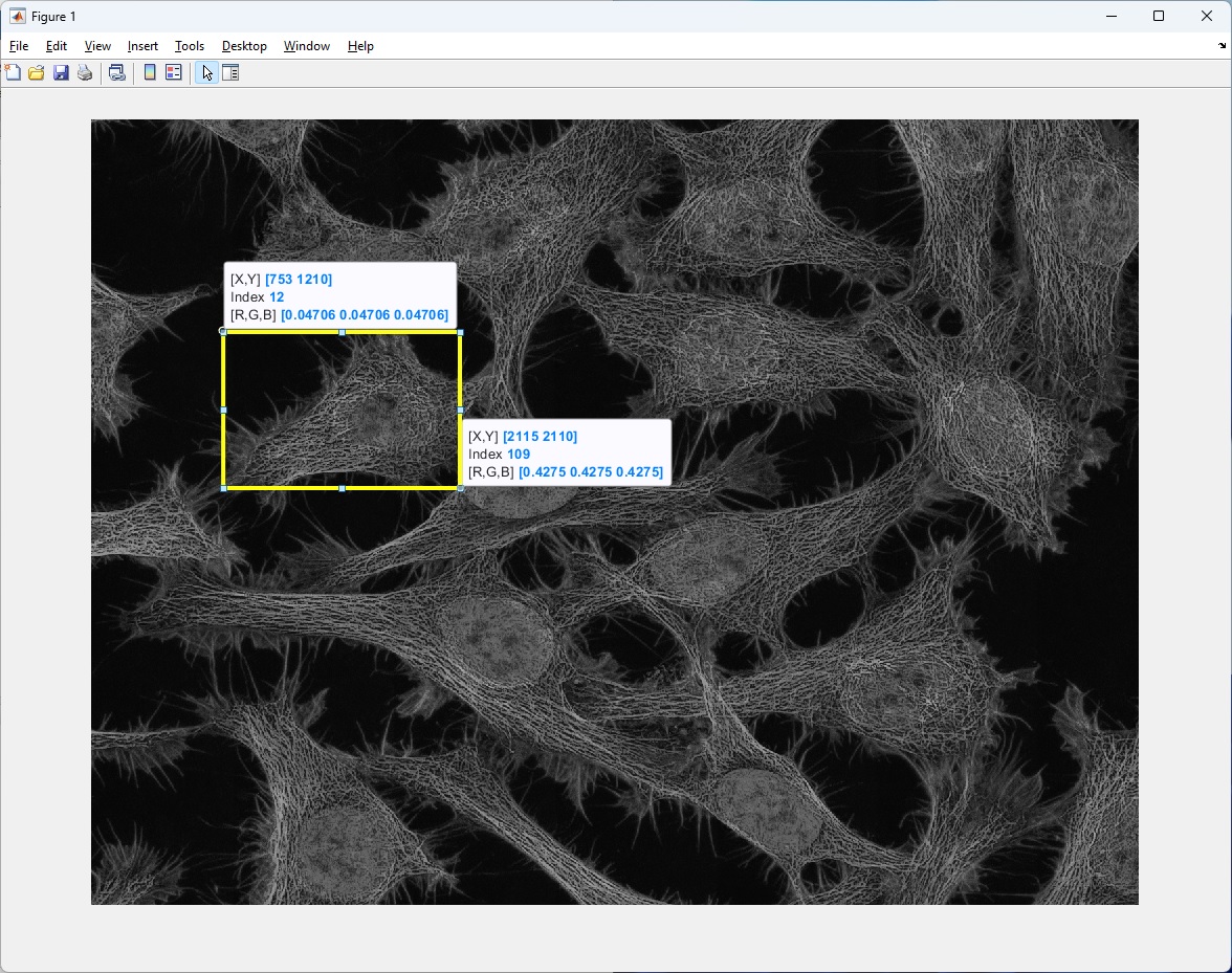
Image processing (영상처리)에서 가장 흔하게 사용되는 기법중의 하나가 이미지

필터링 (image filtering) 입니다. MATLAB에서 기본 제공하는 필터 - Average, Sobel filter 등 -

또는 사용자가 제작한 필터를 이용해 대상 이미지와의 연산(convolution 등)을 통해 새로운

이미지를 생성하는 것을 이미지 필터링(image filtering) 이라고 합니다. 

 

흔히 이미지상의 지정된 부분을 흐릿하게 하거나 대상의 윤곽선(edge)에 강조를 주어 더

선명하게 해주는 기능은 이미지 필터링의 직접적인 역할 입니다.

또한  간접적인 역할로써는, 딥러닝 (deep learning) 네트워크 중 이미지에서 원하는 물체

혹은 대상을 자동으로 검출하는 기능을 하는 CNN (Convolutional Neural Network) 에서의

이미지 데이터는 반드시 한가지 이상의 필터링 과정을 거칩니다.

 

컨볼루션 (convolution) - 여기서는 2D convolution을 예로 들겠습니다 - 은 이미지 필터링의

기본적인 연산 방법으로써, 대상이 되는 데이터의 각 element들과 필터의 각 계수들을

element-wise 곱셈을 하고 그 결과들을 더해서(element-wise sum) 새로운 픽셀 데이터를

얻는 방식입니다. 

 

 

본 글에서는 컨볼루션의 설명을 생략하고 위의 비디오로 (0:33 부터) 대체하겠습니다.

( 위의 비디오 중 컨볼루션 설명 부분은 출처 1 을 참조해 주십시오. )

위의 비디오 (0:33 부터)에서 보듯이, 이미지 필터 - 또는 커널 Kernel, 윈도우 Window 이라고도 합니다 - 를

대상 이미지 데이터의 모든 구역으로 이동하면서 대상 영역의 이웃에 있는 픽셀들과 컨볼루션

연산하는 방식을 선형 공간 필터링 (linear spatial filtering) 이라고 부릅니다. 

 

대상 이미지와 이미지 필터간의 컨볼루션 연산후 결과 데이터의 크기는 줄어들기 때문에

대상 이미지의 테두리를 '0' 값을 가진 픽셀들로 확장 (zero padding) 합니다.

따라서 zero padding에 의해 본래 대상 이미지와 컨볼루션 연산결과의 크기가 같아집니다.

푸리에 변환 (Fourier transform) 을 통한 주파수 도메인 필터링 (Frequency domain filtering) 은

선형 공간 필터링과 구분되는것으로 후에 중급과정에서 다루겠습니다.

 

 

 

Average filtering

 

Average filter는 대상 이미지의 지정된 부분을 흐릿하게 (blur) 하는 역할을 합니다.

필터의 계수는 사용자에 의해 지정된 하나값에 의해 정해지며 그 알고리즘은 간단합니다.

( 밑의 코드중 syntax, algorithm 주석 부분 참조 )

 

예를들어 사용자가 hsize = 3 으로 지정한다면 average filter h는 모든 계수가 1/9이 될 것이고,

이 필터 계수들이 대상 이미지의 픽셀들과 컨볼루션 연산을 수행함으로써 결과 이미지 데이터는

전반적으로 낮은 값을 가지며 흐릿한 영상을 보여줄 것입니다.

 

 

% h = fspecial('average',hsize)  % syntax of built-in filter

% algorithm of built-in filter
% n = (hsize, hsize);
% h = ones(n(1),n(2))/(n(1)*n(2));

n = (3, 3);
h = ones(n(1),n(2)) / (n(1)*n(2)) 

% h = [ 1/9  1/9  1/9 
%       1/9  1/9  1/9 
%       1/9  1/9  1/9 ]

 

 

이번에는 대상 이미지의 특정 cell(세포) 영역을 지정하여 10x10 크기의 average filter를

적용해 보겠습니다.

( 코드에서 쓰인 이미지는 본 블로그 맨밑 출처 2에 가셔서 다운로드 받을 수 있습니다. )

 

 

img = imread('NCI-jdfn7Z03Qa4.jpg');
img_gray = rgb2gray(img);               % convert from RGB to grayscale image data
img_gray = im2double(img_gray);         % convert from uint8 to double type data
img_in = img_gray(1210:2110,753:2115);  % manually set a ROI(regions of interest)

% average filter 
avg_filter = fspecial('average',10);    % a blur filter
img_avg_fil = imfilter(img_in,avg_filter,'replicate','conv');
figure; 
montage({img_in,img_avg_fil}); title('\fontsize{20}Input and (Average) Filtered image');

 

좌: 입력 이미지, 우: average filter가 적용된 이미지

 

 

위의 코드에서 보듯이 fspecial( ) 명령어는 이미지 필터를 만들고, 만들어진 필터를 대상 이미지에

적용하기 위해 imfilter( ) 명령어를 사용하였습니다.

imfilter( )의 부가적인 입력 파라메터로써, 연산방법은 - 필터와 대상 이미지간의 연산 - 컨볼루션 ('conv')

을 이용하고, zero-padding이 아닌 대상 이미지 경계 부분의 마지막 픽셀값을 복제 ('replicate') 및 확장하여

대상 이미지와 필터연산 결과가 같은 크기를 갖도록 하였습니다.

 

기대한바와 같이 필터링의 결과는 입력 이미지에 비해 흐릿한 영상을 보여줍니다.

개인적인 경험상 Neuroscience 분야에서 average filter는 이미지 분석단계에서 자주 사용되지

않았고, 간혹 Image processing(영상처리)의 간단한 전처리(pre-processing)과정 중 노이즈 감소용으로

쓰일때가 있었습니다.

 

 

 

Laplacian filtering

 

Laplacian filter는 기본적으로 high-pass filter로써 주로 사용됩니다.

단조로운 배경에 물체가 하나 있고 이를 푸리에 변환 (fourier transform)을 통해 주파수 도메인

(frequency domain) 에서 보면 물체의 윤곽선(edge)은 갑작스러운 변화로써 고주파 (high frequency)

특성을 갖습니다.

 

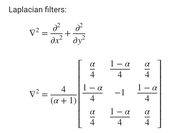
밑의 laplacian filter의 algorithm에서 보듯이 (2차 미분식) 영상신호 기울기의 급격한 변화를

감지하는것이 목적입니다. 그렇기 때문에 laplacian filter는 이러한 고주파 특성, 즉 물체의 윤곽선(edge)을

검출하는데 사용됩니다.

 

필터의 계수는 사용자에 의해 지정된 하나값에 의해 정해지며 그 알고리즘은 다음과 같습니다.

 

 

% h = fspecial('laplacian',alpha)  % syntax of built-in filter

 

Algorithm of laplacian filters (출처3)

 

 

필터의 중앙 계수가 음수이기 때문에 laplacian filtering의 결과 영상이 음수값을 가질수 있습니다. 

따라서 입력 영상 데이터에서 필터 결과 영상을 뺀다면 픽셀값이 증가하여 입력 영상보다 선명해

질수 있습니다. 마찬가지로 특정 cell(세포) 영역을 입력 영상 데이터로써 laplacian filter 를 적용해

보겠습니다.

 

 

img = imread('NCI-jdfn7Z03Qa4.jpg');
img_gray = rgb2gray(img);               % convert from RGB to grayscale image data
img_gray = im2double(img_gray);         % convert from uint8 to double type data
img_in = img_gray(1210:2110,753:2115);  % manually set a ROI(regions of interest)

% laplacian filter 
lap_filter = fspecial('laplacian',0);   % a high-pass filter
img_lap_fil = imfilter(img_in,lap_filter,'replicate','conv');
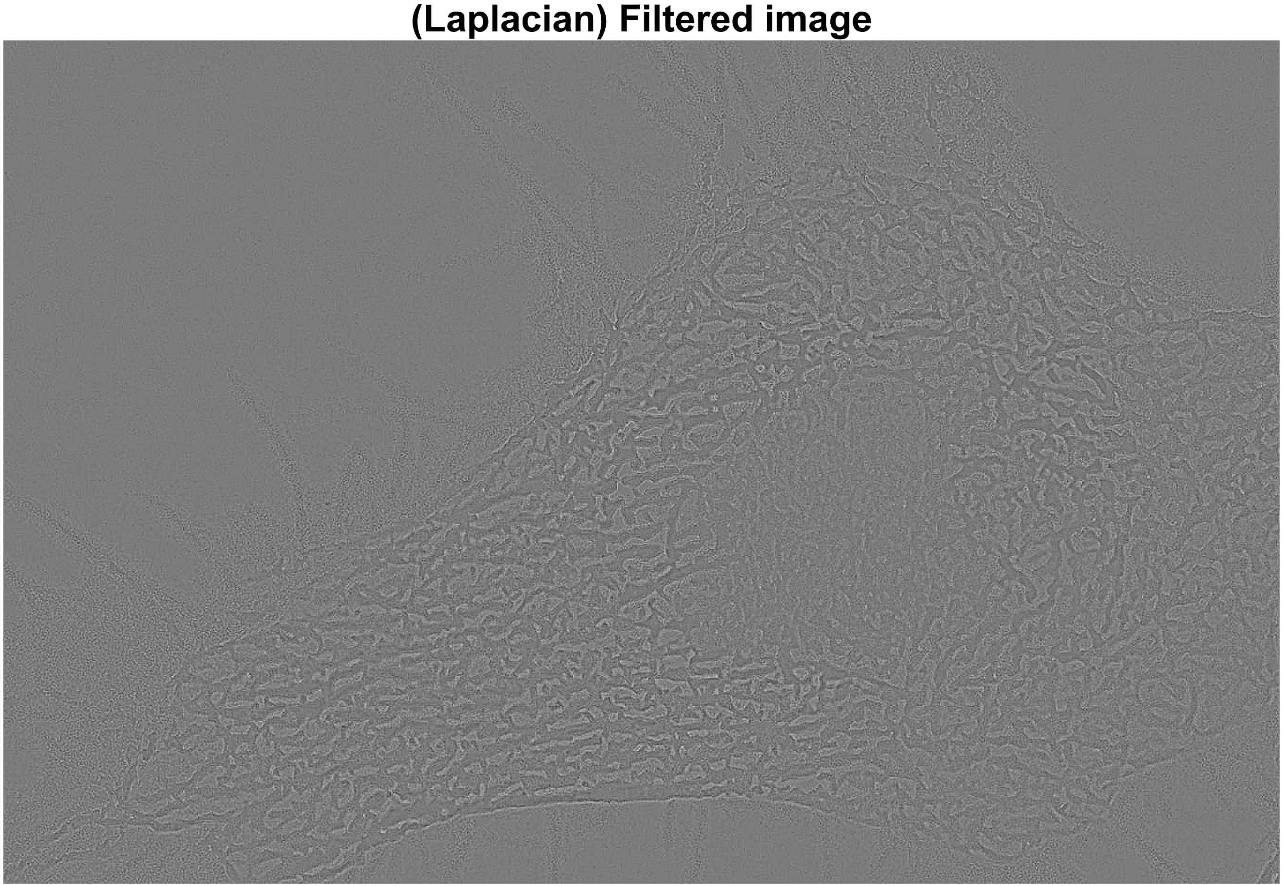
figure; imshow(img_lap_fil,[]); title('\fontsize{20}(Laplacian) Filtered image');
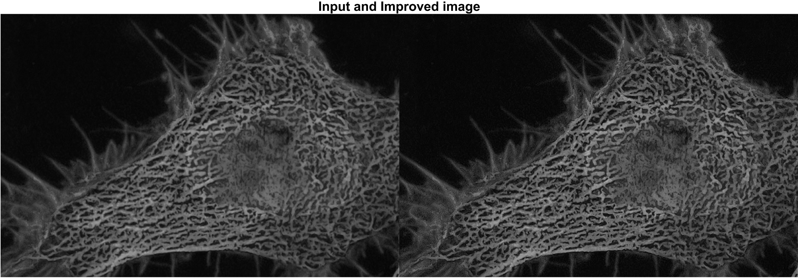
figure; montage({img_in,img_in-img_lap_fil}); title('\fontsize{20}Input and Improved image');

 

 

좌: 입력 이미지, 우: laplacian filter가 적용된 이미지

 

 

위의 코드에서 laplacian filter를 생성할 시 입력 파라메터인 alpha 값을 '0' 으로 지정하였지만,

다른값으로 지정하며 필터링 결과를 비교해 보기를 권해드립니다.

Laplacian filter를 거친 결과 영상 데이터는 음수와 0에 가까운 낮은 픽셀값들을 포함하므로 눈에 띄는

특징을 찾기가 어렵습니다. 하지만 입력 영상과의 (선형연산) 빼기를 통해 원본 보다 cell(세포)의

윤곽선(edge)이 더 뚜렷한 결과 영상 데이터를 가질 수 있습니다.

 

보통 고화질의 Confocal image 또는 Two-Photon image에서는 cell(세포)의 검출 혹은 관찰에 큰 문제가

없었지만 때로는 필터를 이용하여 cell(세포)의 윤곽(edge)에 대한 화질개선을 필요로 하였습니다.  

Laplacian filter는 또다른 윤곽선(edge) 검출 필터인 Sobel filter 보다 더 자주 사용하였습니다.

 

 

 

Sobel filtering

 

Sobel filter 또한 윤곽선(edge)을 검출하는데 많이 사용되는 방법으로써 연산이 간편하다는

장점이 있습니다. Sobel filter는 laplacian filter와 다르게 (1차 미분식) 영상신호 기울기를 측정함

으로써 윤곽선(edge)를 검출합니다.

 

MATLAB에서 제공하는 sobel filter의 계수는 다음과 같습니다.

 

% h = fspecial('sobel')   % syntax of built-in filter

% h = [ 1  2  1           % vertical gradient
%       0  0  0 
%      -1 -2 -1 ]
  
% h = [ 1  0 -1           % horizontal gradient
%       2  0 -2 
%       1  0 -1 ]

 

 

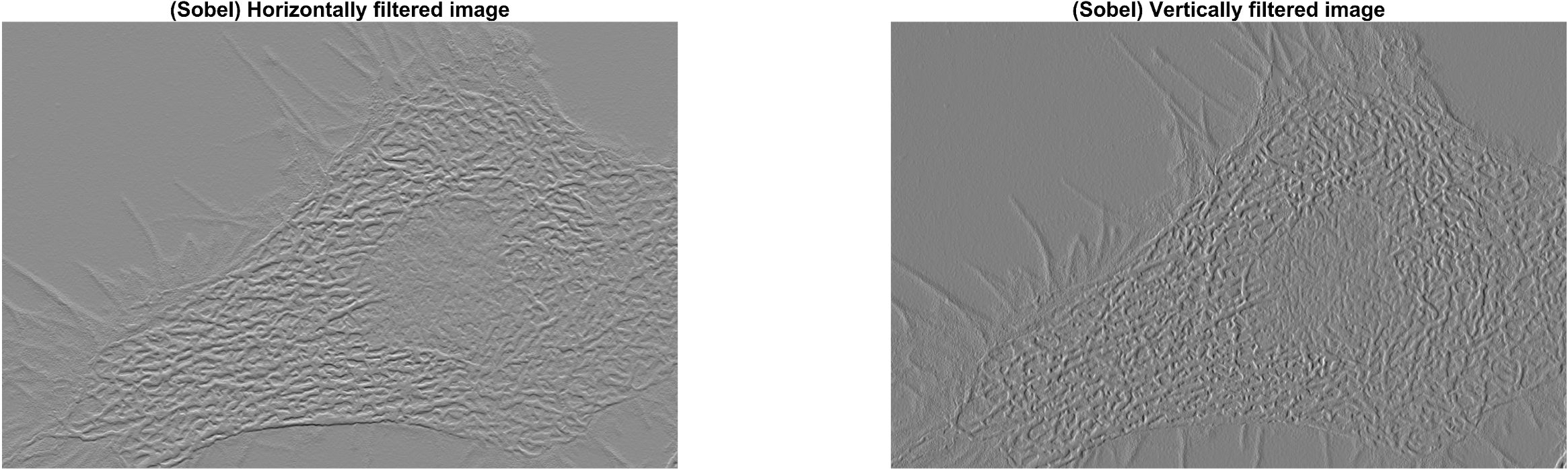
이미지 데이터의 x 혹은 y 방향을 구분지어 필터링을 수행하므로, 필터링의 목적에 맞게끔

필터의 계수를 선택하면 됩니다. 마찬가지로 특정 cell(세포) 영역을 입력 영상 데이터로써

sobel filter 를 x, y 방향에 각각 적용하고, 각각의 필터링 결과를 입력 영상에 더하여(선형 연산)

마지막에 보이겠습니다.

 

img = imread('NCI-jdfn7Z03Qa4.jpg');
img_gray = rgb2gray(img);               % convert from RGB to grayscale image data
img_gray = im2double(img_gray);         % convert from uint8 to double type data
img_in = img_gray(1210:2110,753:2115);  % manually set a ROI(regions of interest)

% sobel filter
sobel_filter = fspecial('sobel');       % horizontal edge detection filter
img_sobel_horizon = imfilter(img_in,sobel_filter,'replicate','conv');
% basically sobel filter emphasizes horizontal edges, and
% it is also able to vertical edges when the filter is transposed
img_sobel_vertical = imfilter(img_in,sobel_filter','replicate','conv'); 
sum_sobel_fil = img_sobel_horizon+img_sobel_vertical;

figure; 
subplot(1,2,1); imshow(img_sobel_horizon,[]); title('\fontsize{20}(Sobel) Horizontally filtered image');
subplot(1,2,2); imshow(img_sobel_vertical,[]); title('\fontsize{20}(Sobel) Vertically filtered image');
figure; montage({img_in+img_sobel_horizon,img_in+img_sobel_vertical}); title('\fontsize{20}Horizontally and Vertically improved image');
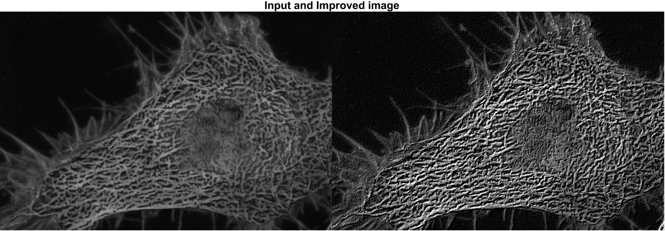
figure; montage({img_in,img_in+sum_sobel_fil}); title('\fontsize{20}Input and Improved image');

 

 

 

좌: Sobel filter가 x축 방향에 적용된 이미지, 우: sobel filter가 y축 방향에 적용된 이미지

 

 

좌: 입력 이미지, 우: (x축 + y축 방향) sobel filter가 적용된 이미지

 

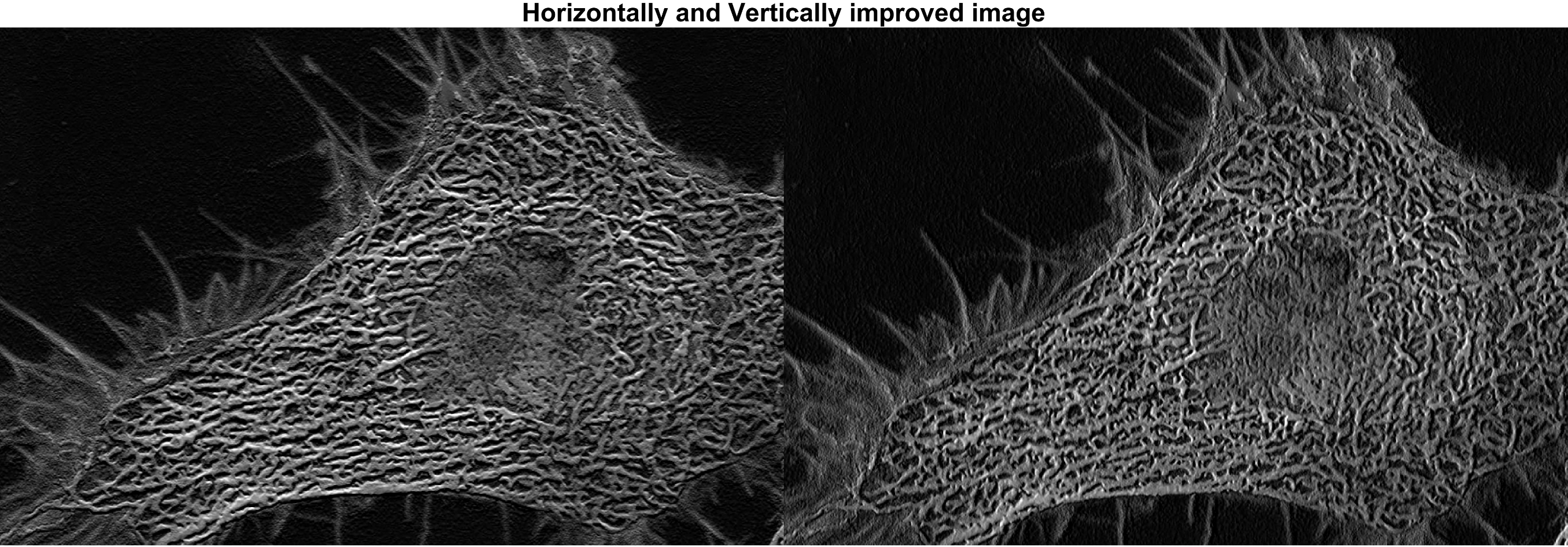
위 중간에 표시된 결과 이미지 (Horizontally and Vertically improved image) 는 

대상 이미지에 각각 x축, y축에 sobel filter 가 적용된 결과를 더하여(선형연산) 얻은 결과 이미지들

입니다. Cell (세포) 내부의 필터링 결과는 비슷해 보이지만 수직 (y축) 으로 뻗은 cell (세포) 바깥부분을 

보면 각 방향에 적용된 필터링의 결과를 비교해 볼수 있습니다.

 

맨 밑의 결과 이미지는 입력 대상 이미지와 x,y 축 모두에 sobel filter 를 적용한 결과 이미지를 비교해

두었습니다.

 

 

 

마지막으로 본 글에 쓰인 모든 MATLAB 코드는 밑에 표시해 두었습니다.

img = imread('NCI-jdfn7Z03Qa4.jpg');
img_gray = rgb2gray(img);               % convert from RGB to grayscale image data
img_gray = im2double(img_gray);         % convert from uint8 to double type data
img_in = img_gray(1210:2110,753:2115);  % manually set a ROI(regions of interest)

% 1) average filter 
avg_filter = fspecial('average',10);    % a blur filter
img_avg_fil = imfilter(img_in,avg_filter,'replicate','conv');
figure; 
montage({img_in,img_avg_fil}); title('\fontsize{20}Input and (Average) Filtered image');

% 2) laplacian filter 
lap_filter = fspecial('laplacian',0);   % a high-pass filter
img_lap_fil = imfilter(img_in,lap_filter,'replicate','conv');
figure; imshow(img_lap_fil,[]); title('\fontsize{20}(Laplacian) Filtered image');
figure; montage({img_in,img_in-img_lap_fil}); title('\fontsize{20}Input and Improved image');


% sobel filter
sobel_filter = fspecial('sobel');       % horizontal edge detection filter
img_sobel_horizon = imfilter(img_in,sobel_filter,'replicate','conv');
% basically sobel filter emphasizes horizontal edges, and
% it is also able to vertical edges when the filter is transposed
img_sobel_vertical = imfilter(img_in,sobel_filter','replicate','conv'); 
sum_sobel_fil = img_sobel_horizon+img_sobel_vertical;

figure; 
subplot(1,2,1); imshow(img_sobel_horizon,[]); title('\fontsize{20}(Sobel) Horizontally filtered image');
subplot(1,2,2); imshow(img_sobel_vertical,[]); title('\fontsize{20}(Sobel) Vertically filtered image');
figure; montage({img_in+img_sobel_horizon,img_in+img_sobel_vertical}); title('\fontsize{20}Horizontally and Vertically improved image');
figure; montage({img_in,img_in+sum_sobel_fil}); title('\fontsize{20}Input and Improved image');

 

 

 

 

출처1: https://www.mathworks.com/discovery/convolution.html

Convolution

 

 

출처2: https://unsplash.com/photos/jdfn7Z03Qa4

사진 작가: National Cancer Institute, Unsplash

 

 

 

출처3: https://www.mathworks.com/help/images/ref/fspecial.html#d124e113760

Create predefined 2-D filter - MATLAB fspecial