[Python 영상처리 기초 8] Affine Transformations

 

 

Affine transformations 은 하나의 이미지 공간에서 다른 공간으로의 매핑으로써

영상처리에서 흔하게 쓰이는 변환중의 하나입니다. 이미지의 확대/축소, 회전,

이동, 반사 등이 affine transformations 의 예입니다.

 

밑의 affine transformation (T) (출처1)에서 보듯이 입력공간 또는 이미지 [x, y]을 대상으로

사용자가 지정한 2x3 크기의 transformatin matrix (M)의 값에 따라 회전, 반사 등의

변환 또는 매핑을 수행할 수 있습니다. 본 포스트에서는 이미지의 (확대/축소를 제외한) 변환을

transformation matrix인 M에 의해 연산할수 있음을 보입니다.

 

 

Affine transformation (출처1)

 

Transformation matrix

 

OpenCV에서의 afffine transformations의 모양은 MATLAB

([MATLAB 영상처리 기초 8] Affine Transformations 참조) 에서의 매트릭스 모양이

다르지만 본질적인 원리는 같습니다.

 

 

 

Translation

 

이미지의 x-, y-축 방향 이동을 위한 transformation matrix를 (출처2) 다음과 같이 지정합니다.

 

 

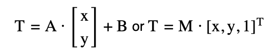
다음은 입력 이미지에서 우측(x축)으로 400 픽셀, 밑(y축)으로 600 픽셀 이동(translate)

하는 예를 보이겠습니다.

 

 

import cv2
import numpy as np
import matplotlib.pyplot as plt
%matplotlib inline

img_color = cv2.imread('national-cancer-institute-jdfn7Z03Qa4-unsplash.jpg',cv2.IMREAD_COLOR)
print("Shape of input image: ",img_color.shape)
row,col,_ = img_color.shape

# translation - move 400px right on x-, move 600px down on y-axis
x_move = 400
y_move = 600

M = np.array([[1, 0, x_move], [0, 1, y_move]]).astype(np.float32)  
t_img = cv2.warpAffine(img_color, M, (col, row))
print("Shape of transformed image: ",t_img.shape)

fig = plt.figure(figsize=(12,10))    
fig.add_subplot(1,2,1)
plt.axis("off")
plt.imshow(cv2.cvtColor(img_color, cv2.COLOR_BGR2RGB))

fig.add_subplot(1,2,2)
plt.axis("off")
plt.imshow(cv2.cvtColor(t_img, cv2.COLOR_BGR2RGB))

plt.show()

 

 

좌: 입력 이미지 (출처3), 우: 우측으로 400픽셀, 밑으로 600픽셀 translation 결과

 

 

이미지의 변환을 수행하는 cv2.warpAffine( ) 메소드의 입력 파라메터 중 변환후

이미지의 크기를 입력 이미지의 크기와 동일하게 지정하였습니다. 그렇기 때문에

translation 변환후의 이미지는 일부가 잘려서 보입니다.

주의할점은 변환후 이미지의 크기를 지정시 (이미지의 폭, 높이) 순서로 명시하여야 합니다.

 

 

 

Scaling

 

다음은 입력 이미지의 확대/축소 입니다. 밑의 변환은 입력 이미지의 x축으로 2배,

y축으로 3배 확대하는 예입니다. OpenCV에서는 transformation matrix (M) 이

아닌 cv2.resize( ) 메소드를 이용하여 이미지의 확대/축소를 할수 있습니다.

 

 

# scaling - enlarge 2x on x-, 3x on y-axis
x_scale = 2
y_scale = 3

t_img = cv2.resize(img_color,None,fx=x_scale, fy=y_scale)
print("Shape of transformed image: ",t_img.shape)

fig = plt.figure(figsize=(12,10))    
fig.add_subplot(1,2,1)
plt.axis("off")
plt.imshow(cv2.cvtColor(img_color, cv2.COLOR_BGR2RGB))

fig.add_subplot(1,2,2)
plt.axis("off")
plt.imshow(cv2.cvtColor(t_img, cv2.COLOR_BGR2RGB))

plt.show()

 

 

좌: 입력 이미지, 우: x축으로 2배, y축으로 3배 scaling 결과

 

 

위의 결과와 같이 입력 이미지의 크기는 4,500 x 6,000 (y-axis, x-axis)이고 출력 이미지의

크기는 13,500 x 12,000 으로써 정확히 x축으로 2배, y축으로 3배 확대 되었습니다.

 

 

 

Rotation

 

다음은 입력 이미지의 회전 변환 입니다. 밑의 변환은 입력 이미지를 기준으로 pi/6 (= 30˚)

만큼 시계방향으로 회전하는 예입니다. 

회전을 위한 보통의 transformation matrix는 밑의 M과 같이 표현하지만 OpenCV에서는

이를 확장하여, 회전중심과 변환결과의 확대/축소가 가능한 매트릭스 메소드를 제공합니다. 

 

변환 매트릭스가 복잡해진 만큼 삼각함수(cosine, sine)값을 직접 transformation matrix에

입력하기 보다는 OpenCV가 제공하는 메소드 - cv2.getRotationMatrix2D( ) - 를 이용

하겠습니다. 입력 파라메터로써 1) 회전중심의 좌표, 2) 회전각도, 3) scale값 들을 차례로 

입력하고, 메소드의 연산결과를 transformation matrix  M으로 지정하면 됩니다.

 

 

Rotation transformation matrix

 

Scaled rotation with adjustable center of rotation

 

 

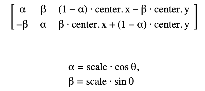
# rotation - -30 degree

# row,col,_ = img_color.shape
center = (col//2, row//2)
angle = -30
scale = 1.0      # optional

M = cv2.getRotationMatrix2D(center, angle, scale)
t_img = cv2.warpAffine(img_color, M, (col, row))

fig = plt.figure(figsize=(12,10))    
fig.add_subplot(1,2,1)
plt.axis("off")
plt.imshow(cv2.cvtColor(img_color, cv2.COLOR_BGR2RGB))

fig.add_subplot(1,2,2)
plt.axis("off")
plt.imshow(cv2.cvtColor(t_img, cv2.COLOR_BGR2RGB))

plt.show()

 

좌: 입력 이미지, 우: 시계방향으로 30˚ rotation 결과

 

 

위 코드에서 보듯이, 이미지의 가운데 픽셀을 회전의 중심으로 지정하였고, 

지정된 회전각도 -30˚는 시계방향으로 30˚ 만큼 회전함을 의미합니다. 

회전된 결과 이미지의 scale은 변하지않게 1.0으로 지정하였습니다.

 

그리고 변환 결과 이미지의 크기 또한 입력 이미지의 크기와 같도록 cv2.warpAffine( )

메소드에 지정하였으므로, 회전변환후 이미지의 일부가 잘려서 보입니다.

 

 

 

Flip

 

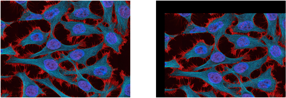
다음은 입력 이미지의 반사 변환 입니다. 밑의 변환은 입력 이미지의 수직선을 기준으로

반사하는 예입니다. 즉, 입력 이미지의 좌우가 바뀌는 결과 이미지를 얻을 수 있습니다.

 

 

# flip - horizontal
# row,col,_ = img_color.shape
M = np.array([[-1, 0, col-1], [0, 1, 0]]).astype(np.float32)
t_img = cv2.warpAffine(img_color, M, (col, row))

fig = plt.figure(figsize=(12,10))    
fig.add_subplot(1,2,1)
plt.axis("off")
plt.imshow(cv2.cvtColor(img_color, cv2.COLOR_BGR2RGB))

fig.add_subplot(1,2,2)
plt.axis("off")
plt.imshow(cv2.cvtColor(t_img, cv2.COLOR_BGR2RGB))

plt.show()

 

 

좌: 입력 이미지, 우: 좌,우의 flip 결과

 

 

입력 이미지의 좌, 우가 반사되었기 때문에 위의 입력, 결과 이미지는 대칭을 이루어

보입니다. 만일 입력 이미지의 수평선을 기준으로 상,하 반사를 하기 위해서는 

transformation matrix를 다음과 설정하면 됩니다.

 

 

# flip - vertical
# row,col,_ = img_color.shape
M = np.array([[1, 0, 0], [0, -1, row-1]]).astype(np.float32)
t_img = cv2.warpAffine(img_color, M, (col, row))

 

 

 

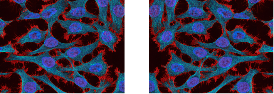
Shear

 

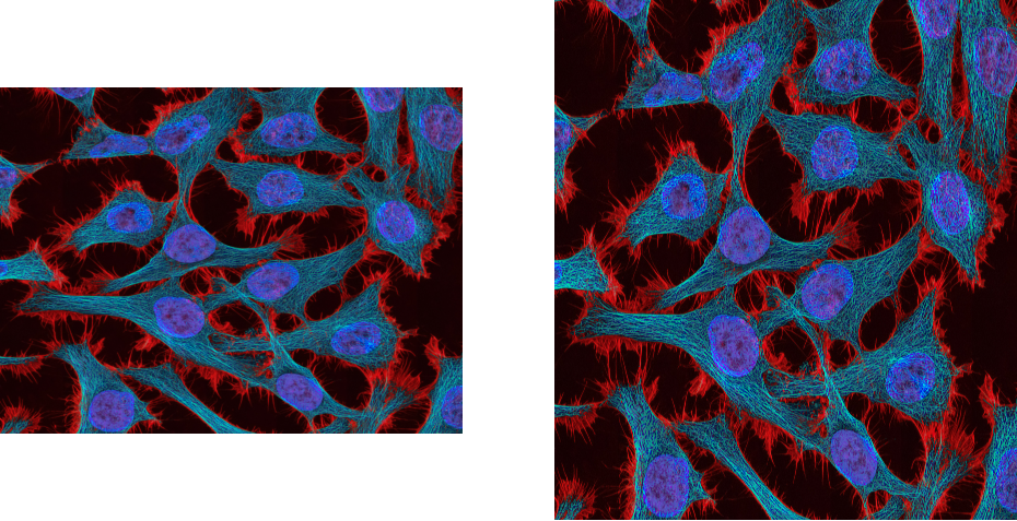
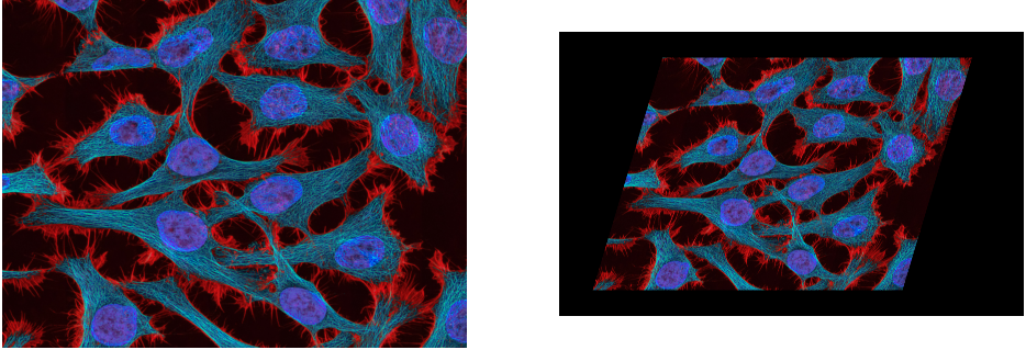
다음은 입력 이미지의 shear 변환 입니다. 이 변환은 마치 이미지의 한 귀퉁이를 

잡아 당기는 듯한 효과를 보여줍니다. 이 변환은 반사(flip) 변환과 같이 수직 또는 수평

두가지 방향으로 나뉘어 변환을 수행합니다.

 

밑의 예는 수평방향으로 0.3 만큼 shear 변환하는 과정입니다. 

 

 

# shear - horizontal
offset = 0.3

M = np.array([[1, -offset, 0], [0, 1, 0]]).astype(np.float32)
t_img = cv2.warpAffine(img_color, M, (col, row))

fig = plt.figure(figsize=(12,10))    
fig.add_subplot(1,2,1)
plt.axis("off")
plt.imshow(cv2.cvtColor(img_color, cv2.COLOR_BGR2RGB))

fig.add_subplot(1,2,2)
plt.axis("off")
plt.imshow(cv2.cvtColor(t_img, cv2.COLOR_BGR2RGB))

plt.show()

 

 

좌: 입력 이미지, 우: 수평방향으로 -0.3 shear 결과

 

 

 

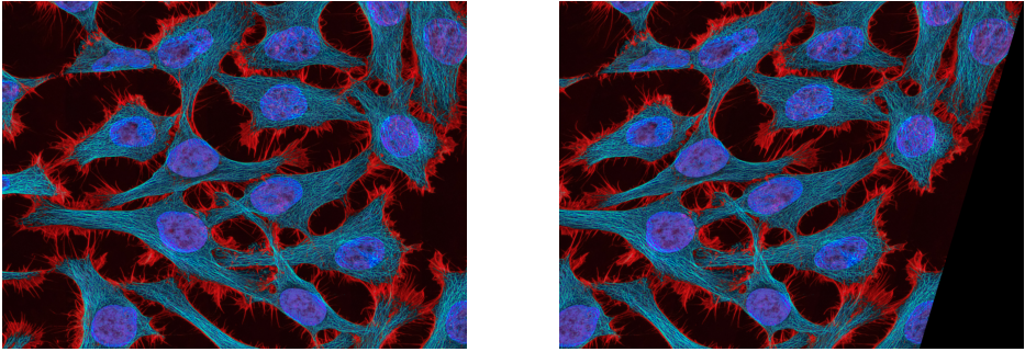
하지만 위 우측의 결과 이미지에서 보듯이 shear 변환의 결과가 뚜렷이 보이지 않습니다.

따라서 입력 이미지에 대한 shear 변환과 동시에 x축으로 2,000 픽셀, y축으로 500 픽셀

translation 변환을 수행하여 결과 이미지를 보겠습니다.

 

cv2.warpAffine( ) 에서 출력 이미지의 크기를 임의로 확장하였습니다.

 

 

x_move = 2000
y_move = 500

M = np.array([[1, -offset, x_move], [0, 1, y_move]]).astype(np.float32)
t_img = cv2.warpAffine(img_color, M, (col+3000, row+1000))
print("Shape of transformed image: ",t_img.shape)

fig = plt.figure(figsize=(12,10))    
fig.add_subplot(1,2,1)
plt.axis("off")
plt.imshow(cv2.cvtColor(img_color, cv2.COLOR_BGR2RGB))

fig.add_subplot(1,2,2)
plt.axis("off")
plt.imshow(cv2.cvtColor(t_img, cv2.COLOR_BGR2RGB))

plt.show()

 

 

좌: 입력 이미지, 우: 수평방향으로 -0.3 shear 및 translation 결과

 

 

 

같은 방식으로 수직방향으로 shear 변환을 하고자 한다면 밑의 코드와

같습니다. 

 

 

# shear - vertical
offset = 0.3

M = np.array([[1, 0, 0], [-offset, 1, 0]]).astype(np.float32)
t_img = cv2.warpAffine(img_color, M, (col, row))

 

 

 

 

 

 

출처1: https://docs.opencv.org/3.4/d4/d61/tutorial_warp_affine.html

OpenCV: Affine Transformations

 

 

 

 

출처2: https://docs.opencv.org/4.x/da/d6e/tutorial_py_geometric_transformations.html

OpenCV: Geometric Transformations of Images

 

 

 

 

출처3: https://unsplash.com/photos/jdfn7Z03Qa4

사진 작가: National Cancer Institute, Unsplash