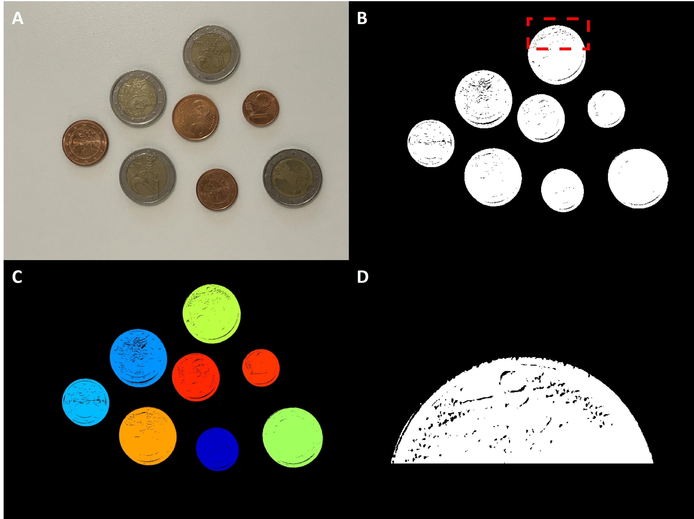
이번에는 동전들이 포개어지거나 겹쳐있지 않고 서로 떨어진 입력 이미지를 다루어 보겠습니다.
입력 이미지는 밑의 [그림 1] 이미지 모음중 A에 표시되었고 배경이 밝기 때문에 이를 Otsu
thresholding 로써 BW이미지로 변환후 픽셀들을 inverse 하였습니다 (B에 표시).
각각의 동전들은 BW이미지에서 쉽게 구분이 되기 떄문에, 이에대한 connected components를
찾는것 또한 쉽습니다. bwconncomp( ) 함수의 입력 파라메터 conn=8로써 적용한 objects 검출
결과는 C에 보여지고 있습니다.
( bwconncomp( )와 labelmatrix( )에 대한 설명은 앞선글 [MATLAB 영상처리 기초9] BW 이미지의 Objects 다루기 1
를 참조해 주십시오 )
B의 상단에 위치한 동전에 빨간색 네모상자 부분을 확대하여 D에 보이고 있습니다. 보시다시피
동전의 윤곽선은 매끄럽지 못하고, 동전 부분에 여러 빈틈이 보입니다.
이로써 입력 이미지 A에 대한 objects segmentation이 간단히 진행되었고, 이를 바탕으로 다양한
종류의 morphologicla operations 들을 나열하는 방식으로 소개 하겠습니다.
% coin segmentation
img = imread('coin_spread.jpg');
img_gray = im2double(rgb2gray(img));
img_BW = ~imbinarize(img_gray);             % inverse BW

% find and count connected components in binary image
cc8 = bwconncomp(img_BW,8);
label8 = labelmatrix(cc8);
img_label8 = label2rgb(label8,'jet','k','shuffle');

% choose a coin and zoom-in its boundary
y_range = 178:546;                          % input [y-,x-coordinate] manually
x_range = 1994:2858;
coin_bound = img_BW(y_range,x_range);

figure; montage({img,img_BW,img_label8,coin_bound})
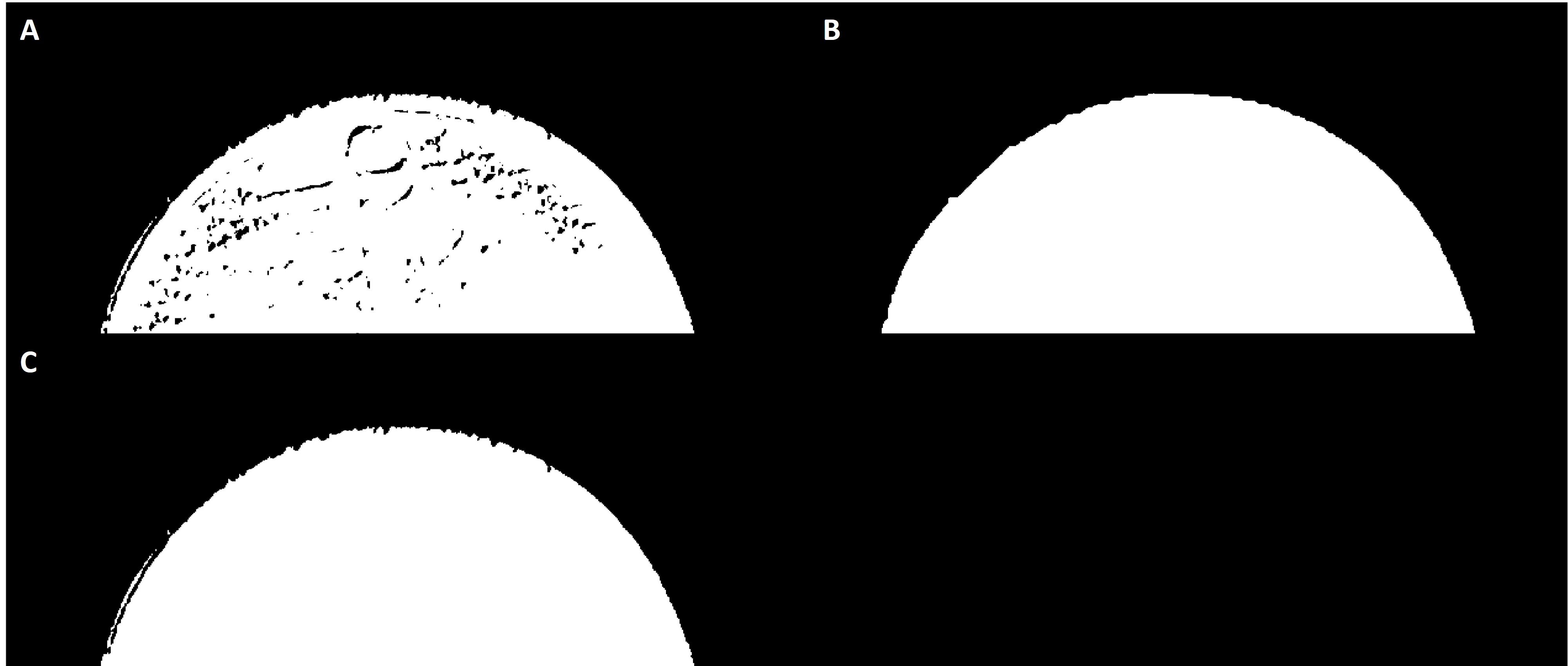
Fill image regions and holes
앞선글 [MATLAB 영상처리 기초 9] BW 이미지의 Objects 다루기 2 에서 언급한 것과 같이
morphological closing (형태학적 닫기) 는 대상 이미지를 dilation 하고 난후, erosion을 수행함
으로써 대상 이미지 objects의 작은틈을 채우고 윤곽선을 부드럽게 하는 효과를 보입니다.
입력 이미지 A (위의 [그림 1] objects segmentation 이미지중 D와 같음) 를 상대로 형태학적 닫기를
수행한 결과가 B에 나타내고 있습니다. 동전의 윤곽선은 다소 부드러워 졌고 동전의 빈틈은 전부
'1'로써 채워졌음을 알 수 있습니다. 형태학적 닫기를 위해 지름이 30픽셀인 disk 모양의 structuring
element가 이용되었고, 이것의 크기, 모양 혹은 반복횟수를 다르게 적용하면 동전의 윤곽선이 좀 더
부드러워 질 수 있을것입니다.
Objects의 빈틈을 채우는 기능만을 필요로 한다면 imfill( ) 명령어를 사용할 수 있습니다. 이것은 입력
파라메터에 따라 objects의 빈틈을 일괄적으로 채울뿐만 아니라 사용자가 지정한 특정위치에서도
빈틈을 채우는 기능을 갖고 있습니다.
img = imread('coin_spread.jpg');
img_gray = im2double(rgb2gray(img));
img_BW = ~imbinarize(img_gray);             % inverse BW

% choose a coin and zoom-in its boundary
y_range = 178:546;                          % input [y-,x-coordinate] manually
x_range = 1994:2858;

% morphological operations
% 1) morphological closing
se_disk30 = strel('disk',30);
imgC_disk30 = imclose(img_BW,se_disk30);

% 2) fill image regions and holes
img_fill = imfill(img_BW,'holes');
figure; montage({coin_bound,imgC_disk30(y_range,x_range),img_fill(y_range,x_range)})
Remove small objects from binary image
위의 [그림 1] objects segmentation 중에서 D 이미지를 좀 더 확대하면 밑의 [그림 3]의 A와 같고,
빨간색 타원형의 범위안에 작은 object가 존재함을 볼 수 있습니다. 이는 입력 이미지의 binarization
(이진화) 과정중에 생긴것으로 노이즈 혹은 불필요한것으로 제거대상일 수 있습니다.
bwareaopen( ) 명령어는 BW이미지를 상대로 사용자에 의해 지정된 크기 보다 작은 objects를 제거하는
역할을 합니다.
이 명령어를 이용하여 크기(object의 픽셀수 총합) 가 100보다 작은 object를 제거한 결과가 밑의
[그림 3] B에 보여지고 있습니다. A와 B 같은 위치의 빨간색 타원안을 비교하면 결과를 알 수 있습니다.

img = imread('coin_spread.jpg');
img_gray = im2double(rgb2gray(img));
img_BW = ~imbinarize(img_gray);             % inverse BW

% choose a coin and zoom-in its boundary
y_range = 178:546;                          % input [y-,x-coordinate] manually
x_range = 1994:2858;

% morphological operations
% 3) remove small objects from binary image
img_ao = bwareaopen(img_BW,100,4);
figure; montage({img_BW(y_range,x_range),img_ao(y_range,x_range)})
Objects' boundaries
Objects들의 윤곽선(= boundary)을 따라 다양한 색상으로써 선을 그리고 objects 내부를 색으로
채우는 연산을 수행하겠습니다.
입력 이미지로써 위의 [그림 2] Object에 imclose( )한 결과를 사용할 것이고, 밑의 [그림 4] A에
보여지고 있습니다. 그리고 이것을 bwboundaries( ) 함수의 입력 파라메터로써 연산을 한다면,
이 함수는 1) cell 형식의 윤곽선 좌표(x-, y-axis)와 2) ([그림 1]의 C와 같은) objects의 label을 결과
로써 반환합니다.
그러므로 밑의 [그림 4] B와 같이 objects 내부를 다양한 색상으로 채우고, boundary를 하얀색 선으로
그려 objects에 하이라이트를 줄 수 있습니다.

img = imread('coin_spread.jpg');
img_gray = im2double(rgb2gray(img));
img_BW = ~imbinarize(img_gray);             % inverse BW

% choose a coin and zoom-in its boundary
y_range = 178:546;                          % input [y-,x-coordinate] manually
x_range = 1994:2858;

% morphological operations
% 1) morphological closing
se_disk30 = strel('disk',30);
imgC_disk30 = imclose(img_BW,se_disk30);

% 4) show objects' boundaries
[BW_bound,label_bound] = bwboundaries(imgC_disk30,'noholes');
fig = figure; imshow(label2rgb(label_bound, @jet, [.5 .5 .5]),'Border','tight')
hold on
for iter = 1:length(BW_bound)
   boundary = BW_bound{iter};
   plot(boundary(:,2), boundary(:,1), 'w', 'LineWidth', 3)
end
img_BW_bound = getframe(fig);
close(fig)
figure; montage({imgC_disk30,img_BW_bound.cdata})
Usage of regionprops( )
BW이미지 objects들의 기준점 혹은 중간점(= centroids)을 구하고 이를 바탕으로 각 object의 면적
(= 각 object 픽셀의 총합)을 얻을 수 있으며 그 외에도 object 면적의 특징에 기반한 여러가지 연산이
가능합니다. 이러한 연산은 바로 regionprops( ) 명령어 하나로써 수행될 수 있습니다.
( 반드시 MATLAB의 help 에서 다양한 기능을 확인해 보시기 바랍니다 )
밑의 [그림 5]의 A에는 각 동전의 centroid를 빨간색 별모양의 마커로써 표시하였습니다.
각 object들이 원형이므로 균형있는 centroid를 보이고 있습니다.
그리고 [그림 5]의 B에는 각 동전의 영역을 포함하는 - 윤곽선이 아닌 - 최소 크기의 네모상자가 objects를
표시하고 있습니다. 이것을 bounding box라고 부르며, 대상 이미지의 object segmentation/extraction
수행시 결과물에 하이라이트를 줄 수 있는 기능 입니다.

img = imread('coin_spread.jpg');
img_gray = im2double(rgb2gray(img));
img_BW = ~imbinarize(img_gray);             % inverse BW

% morphological operations
% 1) morphological closing
se_disk30 = strel('disk',30);
imgC_disk30 = imclose(img_BW,se_disk30);

% 5) usage of regionprops - i) area of objects each
coin_area = regionprops(imgC_disk30, 'Area');

% ii) centroid of objects
coin_centroid = regionprops(imgC_disk30,'centroid');
coin_centroid = cat(1, coin_centroid.Centroid);
fig = figure; imshow(imgC_disk30,'Border','tight')
hold on
plot(coin_centroid(:,1),coin_centroid(:,2), 'r*','MarkerSize',13)
hold off
img_BW_cent = getframe(fig);
close(fig)

% iii) bounding box
% [x y width height] of bounding box' upper-left corner
coin_box = regionprops(imgC_disk30,'BoundingBox');
fig = figure; imshow(imgC_disk30,'Border','tight'); hold on
for box_iter = 1:1:numel(coin_box)
    rectangle('Position',coin_box(box_iter).BoundingBox,'EdgeColor','b',...
    'LineWidth',3);
end
hold off
img_BW_boundBox = getframe(fig);
close(fig)

figure; montage({img_BW_cent.cdata,img_BW_boundBox.cdata})
마지막으로 본 글에 쓰인 모든 MATLAB 코드는 밑에 표시해 두었습니다.
%% coin segmentation

img = imread('coin_spread.jpg');
img_gray = im2double(rgb2gray(img));
img_BW = ~imbinarize(img_gray);             % inverse BW

% find and count connected components in binary image
cc8 = bwconncomp(img_BW,8);
label8 = labelmatrix(cc8);
img_label8 = label2rgb(label8,'jet','k','shuffle');

% choose a coin and zoom-in its boundary
y_range = 178:546;                          % input [y-,x-coordinate] manually
x_range = 1994:2858;
coin_bound = img_BW(y_range,x_range);

figure; montage({img,img_BW,img_label8,coin_bound})

%% morphological operations

% 1) morphological closing
se_disk30 = strel('disk',30);
imgC_disk30 = imclose(img_BW,se_disk30);

% 2) fill image regions and holes
img_fill = imfill(img_BW,'holes');
figure; montage({coin_bound,imgC_disk30(y_range,x_range),img_fill(y_range,x_range)})

% 3) remove small objects from binary image
img_ao = bwareaopen(img_BW,100,4);
figure; montage({img_BW(y_range,x_range),img_ao(y_range,x_range)})

% 4) show objects' boundaries
[BW_bound,label_bound] = bwboundaries(imgC_disk30,'noholes');
fig = figure; imshow(label2rgb(label_bound, @jet, [.5 .5 .5]),'Border','tight')
hold on
for iter = 1:length(BW_bound)
   boundary = BW_bound{iter};
   plot(boundary(:,2), boundary(:,1), 'w', 'LineWidth', 3)
end
img_BW_bound = getframe(fig);
close(fig)
figure; montage({imgC_disk30,img_BW_bound.cdata})

% 5) usage of regionprops - i) area of objects each
coin_area = regionprops(imgC_disk30, 'Area');

% ii) centroid of objects
coin_centroid = regionprops(imgC_disk30,'centroid');
coin_centroid = cat(1, coin_centroid.Centroid);
fig = figure; imshow(imgC_disk30,'Border','tight')
hold on
plot(coin_centroid(:,1),coin_centroid(:,2), 'r*','MarkerSize',13)
hold off
img_BW_cent = getframe(fig);
close(fig)


% iii) bounding box
% [x y width height] of bounding box' upper-left corner
coin_box = regionprops(imgC_disk30,'BoundingBox');
fig = figure; imshow(imgC_disk30,'Border','tight'); hold on
for box_iter = 1:1:numel(coin_box)
    rectangle('Position',coin_box(box_iter).BoundingBox,'EdgeColor','b',...
    'LineWidth',3);
end
hold off
img_BW_boundBox = getframe(fig);
close(fig)

figure; montage({img_BW_cent.cdata,img_BW_boundBox.cdata})
출처1: 본 블로그의 작성자 직접 촬영. 학술/상업적 자유롭게 사용 가능.
https://drive.google.com/file/d/12iuuxdnJ8l7A3_HkmVL45I6Y6PXEVWTS/view?usp=drive_link