[MATLAB 영상처리 기초 3] 이미지의 픽셀값 다루기 - RGB2Gray, Histogram, Binarization(global & adaptive thresholding)

 

 

 

컬러이미지의 grayscale 변환 및 histogram 소개 동영상

 

 

 

픽셀 (pixel)은 이미지를 구성하는 기본요소로써 한 그룹의 픽셀들이 점, 선, 면 등을 나타낼 수 있고,

각 픽셀 값에 의해 이미지의 밝기, 명암 등을 나타낼 수 있습니다.  (모자이크가 좋은 예 입니다.)

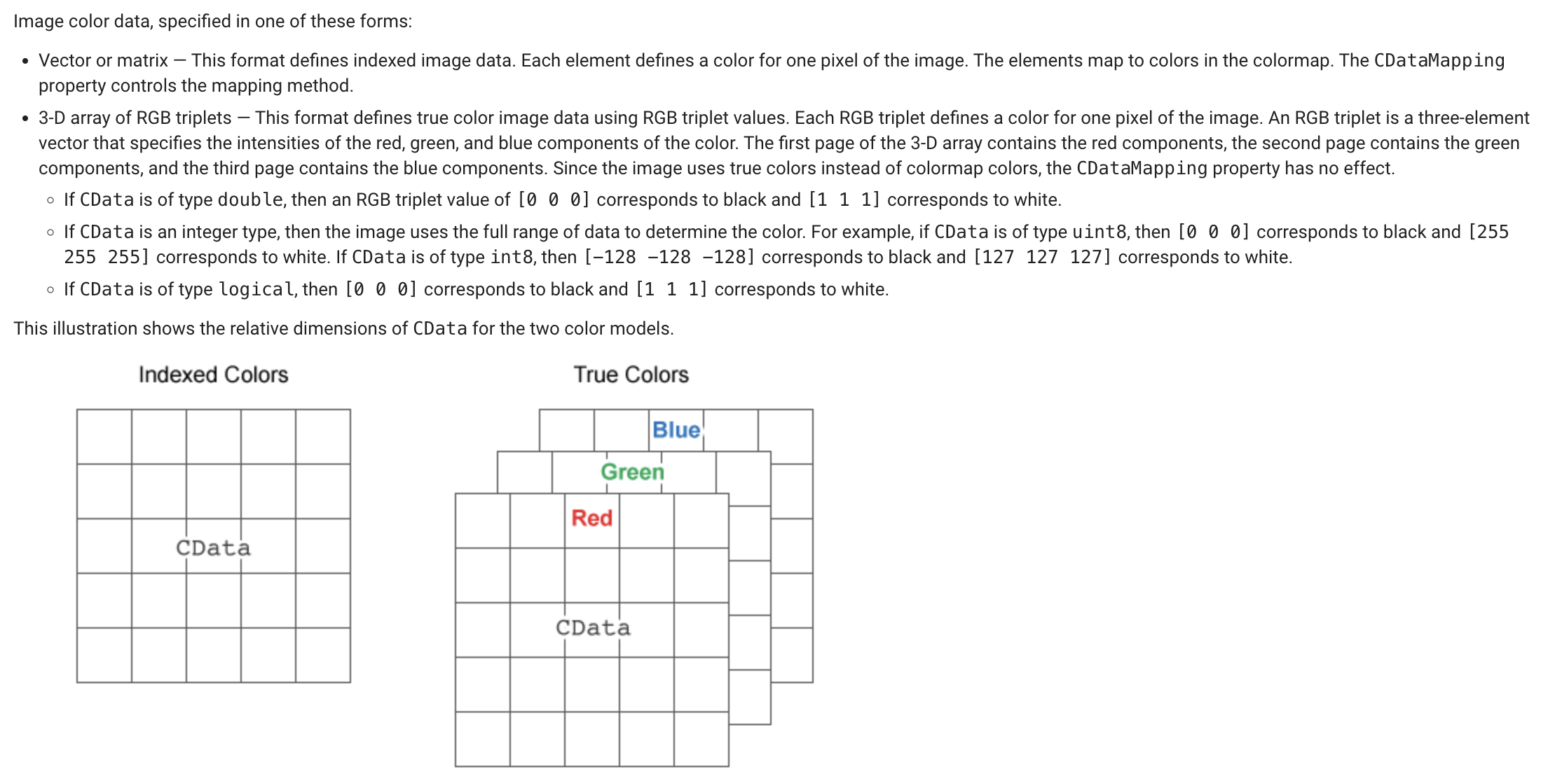
이미지 데이터는 높이(세로) x 폭(가로)의 2차원, 혹은 높이(세로) x 폭(가로) x 색상채널의 3차원

픽셀값 모임이라고 볼 수 있습니다. 

 

3차원 이미지 데이터의 구조는 아래의 그림에 묘사되어 있으며, 앞선 글에서 대상이 되는 3차원의

RGB컬러 이미지 파일을 MATLAB의 workspace 에 불러들여 Red, Green, Blue 각각의 색상채널로

분리하는것을 수행하였습니다. 

 

대상 이미지의 픽셀값은 - MATLAB에서 기본적으로 - uint8(부호없는 8비트 정수형) 형식을 따르며

이는 최소 0 부터 최대 255까지 256가지 범위를 갖습니다. 하나의 픽셀에 빨강, 초록, 파랑의 3개 

채널 intensity를 갖으므로 이들의 조합으로 인해 다양한 색상 스펙트럼을 갖습니다. 

 

 

Image Properties in MATLAB (출처 1)

 

 

Grayscale 이미지로 변환 - RGB2Gray( )

 

이번 글에서는 3차원의 컬러가 아닌 2차원의 grayscale 이미지 데이터를 다룹니다.

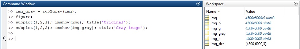
앞선 글에서와 같이 컬러 이미지 파일은 이미 "img" 라는 변수에 저장되어 있습니다.

본 글에 쓰인 이미지는 본 블로그 맨밑 출처 2에 가셔서 다운로드 받을 수 있습니다.

 

img = imread('NCI-jdfn7Z03Qa4.jpg');
img_gray = rgb2gray(img);

figure;
subplot(1, 2, 1); imshow(img); title('Original');
subplot(1, 2, 2); imshow(img_gray); title('Gray image');

 

 

 

좌측 Original: Cells from cervical cancer - National Cancer Institute (출처2)

 

 

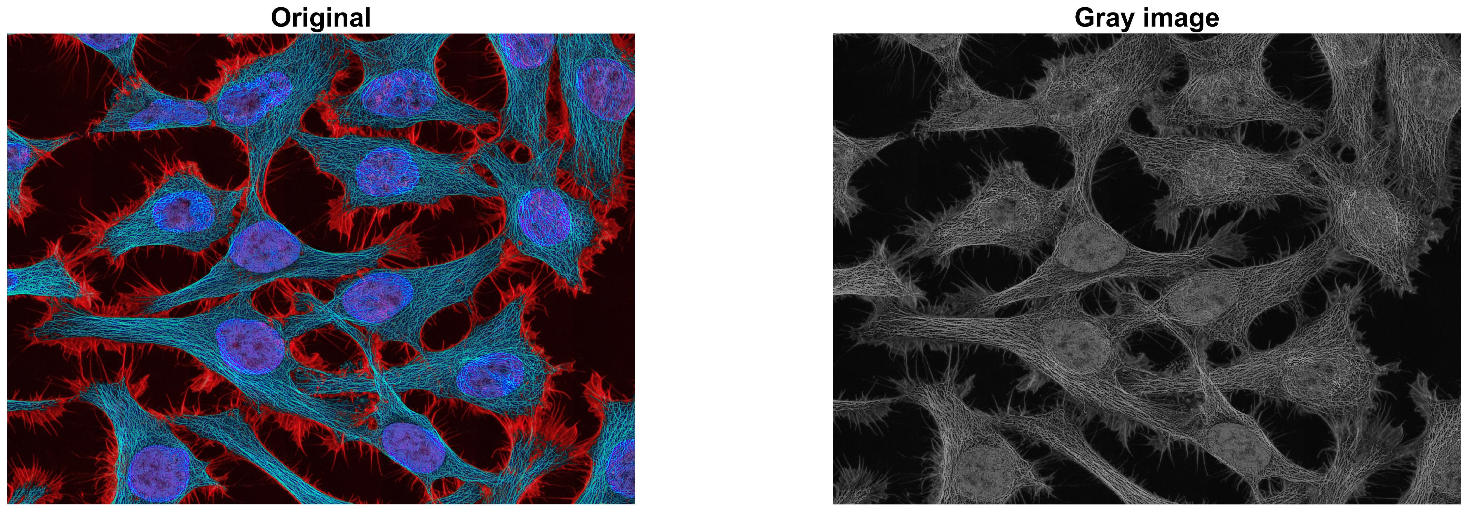
우측의 gray scale 이미지에서 보이듯이 cell(세포)의 특정 염색 색상정보는 사라졌고, 

픽셀값에 의해 cell(세포)의 윤곽과 어두운 명암비가 나타남을 알수 있습니다. 

 

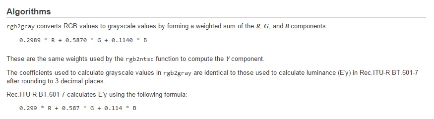
한 발 더 나아가, grayscale 이미지 변환의 알고리즘은 MATLAB의 help에 설명이 되어 있습니다.

( MATLAB 툴바에 물음표 모양의 아이콘을 클릭하면 help 창이 열리며, 검색에서 rgb2gray를 입력하면

상세정보가 나옵니다. ) 

밑의 설명과 같이 각 색상채널의 픽셀값에 특정한 가중치를 곱하여 gray scale 이미지로 변환됨을

알 수 있습니다. 

 

 

rgb2gray( ) algorithms (출처 3)

 

 

 

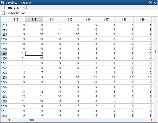
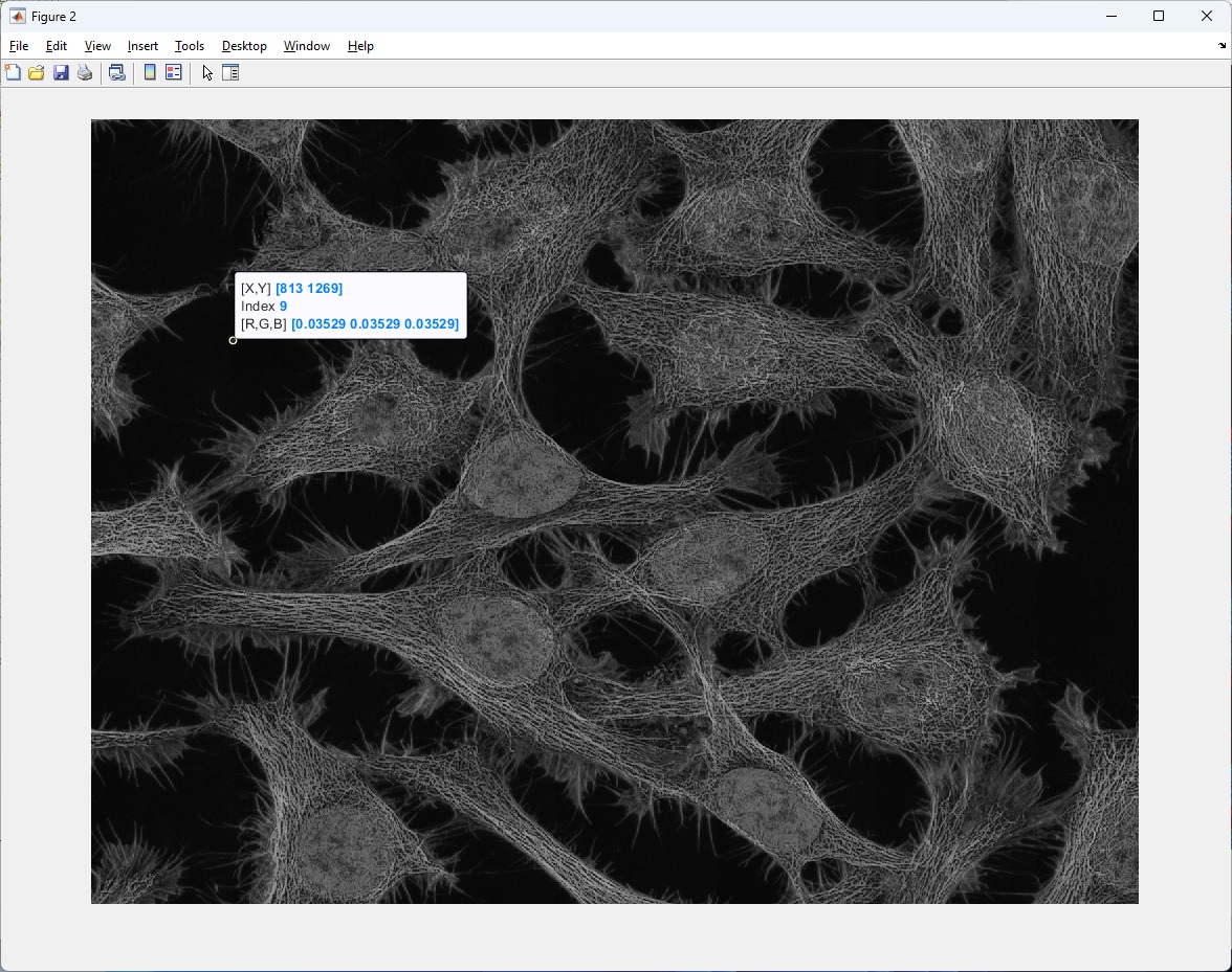
Grayscale 이미지의 바탕이 되는 배경은 검은색으로 보이지만 실제로도 픽셀값 0을 갖는 검은색일까?

특정 픽셀값을 알고자 하면 workspace의 대상 변수를 더블클릭 하여 알수 있으며 또한 Figure의 툴메뉴

중 Data Cursor를 통해 알 수도 있습니다.

( Figure 창에서 Tools -> Data Cursor. 본 글의 맨위에 게시된 동영상 참조 )

 

예를들어, 그레이스케일 이미지의 1269행 813열의 픽셀값은 uint8 형식의 9 입니다.

( 다른 표현으로  img_gray[1269, 813] = 9 )

 

 

 

Data Cursor에 의한 특정 픽셀 정보 참조

 

 

Grayscale 이미지의 픽셀값 중 최소(min), 최대(max), 중간값(median) 은 

 

min(img_gray(:))              % select all element. img_gray(:)
max(img_gray(:))
median(img_gray(:))

 

 

 

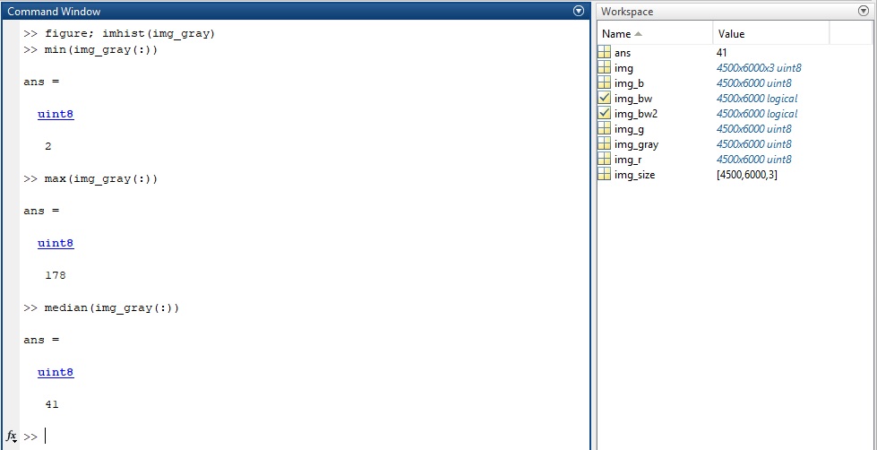
위의 코드에서 grayscale 이미지는 2차원 데이터 이므로 연산 범위를 데이터 전체로 지정하여야 합니다.

만일, 범위지정 없이 명령문을 수행하면, 예를들어  min( img_gray ) 은 각 차원의 최소값을 나타낼 것입니다.

 

 

 

Histogram - imhist( )

 

앞서 언급한 바와 같이 위의 grayscale 이미지 데이터는 uint8 형식(부호없는 8비트 정수형) 이므로 픽셀값은

최소 0 부터 최대 255 까지 256 가지의 범위를 갖습니다.

이미지상의 픽셀값 분포를 알고자 한다면 Histogram이 유용할 것입니다.

또한 histogram은 앞으로 본 블로그에서 소개할 이미지의 콘트라스트 개선(contrast adjustment)이나

이진화(binarization) 등에 유용하게 사용됩니다.

 

figure;
imhist(img_gray);

 

 

 

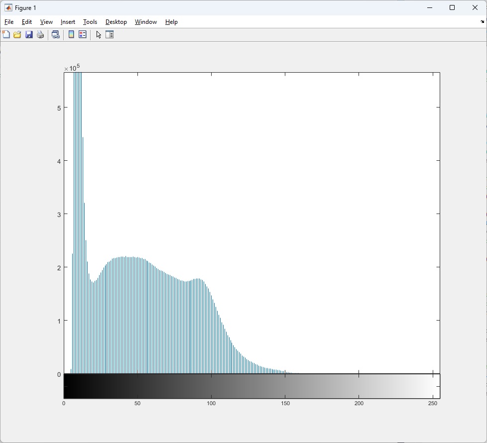
Histogram의 x축은 픽셀값 범위 0 부터 255를 나타내며, y축은 각 픽셀값 (혹은 bin 이라고도 함)

에 해당하는 픽셀의 갯수(frequency 라고도 )를 나타냅니다.

 

만일 픽셀값의 분포가 균일하다면 histogram의 막대(frequency) 높이는 비슷하겠지만, 

위의 histogram에서 보듯이 픽셀값의 분포가 낮은값에 치우쳤고 오른쪽에 긴꼬리(= positively skewed)

를 갖고 있음을 알 수 있습니다. 이것은 이미지 밝기(brightness)가 어두운 부분이 밝은 부분보다

상대적으로 더 많이 분포해 있음을 뜻합니다.

 

MATLAB에서 histogram의 입력 데이터는 반드시 grayscale 또는 2차원의 이미지 데이터 이어야함에 주의하십시오.

 

 

 

 

- YouTube

 

 

 

 

 

이미지의 이진화(Binarization) - global thresholding with Otsu algorithm

 

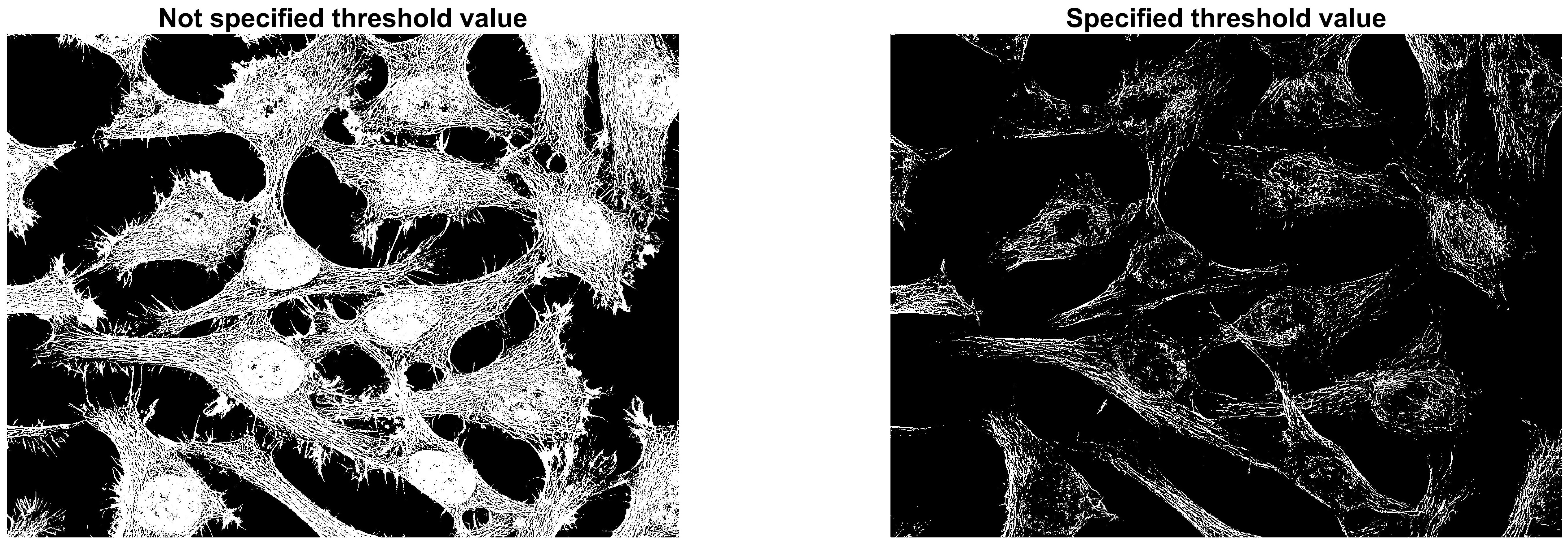
Grayscale 이미지의 픽셀값이 특정 값(= threshold 혹은 임계값) 보다 작거나 같으면 0,

크면 1 을 갖는 이진화 이미지로 변환하는 것을 global thresholding 이라고 합니다. 

여기에서 변환의 기준이 되는 특정 값인 threshold 를 이용하는 것은 binarization의 가장

기초가 되는 방식입니다.

 

MATLAB에서는 binarization의 기본방식으로 Otsu 알고리즘을 이용합니다. 

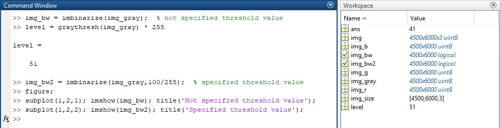
imbinarize( ) 함수는 이진화 이미지 만을 결과로 돌려주기 때문에 Otsu 알고리즘에 의한

threshold는 graythresh( ) 함수를 이용해 알 수 있습니다.

밑의 코드의 "level" 은 정규화된 0과 1 사이의 값이므로, 255을 곱해 uint8 형식으로 변환

하였습니다.

 

만일 원하는 threshold가 있다면 imbinarize( ) 함수의 입력 파라메터로 지정할 수 있습니다.

여기에서는 threshold = 100 을 uint8 타입의 최대값 255으로 나누어 0과 1 사이의

값으로써 정규화 하여 입력 파라메터를 지정하였습니다. 

 

 

img_bw = imbinarize(img_gray);               % default method: Otsu algorithm
level = graythresh(img_gray) * 255           % level is a threshold Otsu algorithm operated
img_bw2 = imbinarize(img_gray, 100/255);     % giving a specified threshold 

figure;
subplot(1, 2, 1); imshow(img_bw); title('Not specified threshold value');
subplot(1, 2, 2); imshow(img_bw2); title('Specified threshold value');

 

 

 

 

 

좌: Otsu, 우: 특정 threshold를 적용한 global thresholding 결과 이미지

 

 

 

Otsu 알고리즘에 대해 알고 싶다면 구글링이나 밑의 페이퍼를 참조해 주십시오.

 

 

 

 

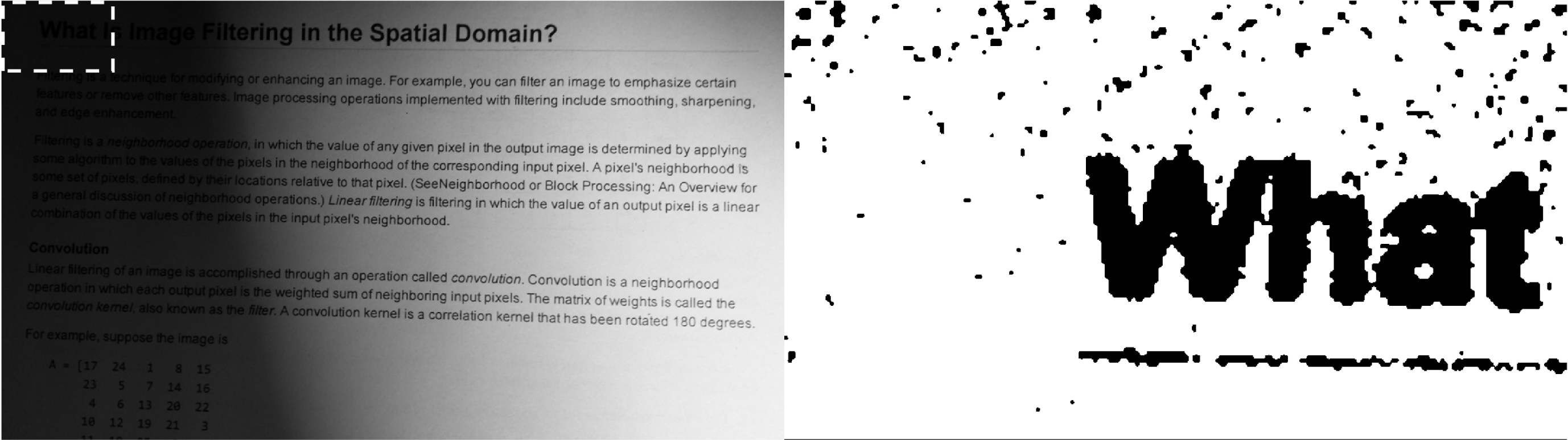
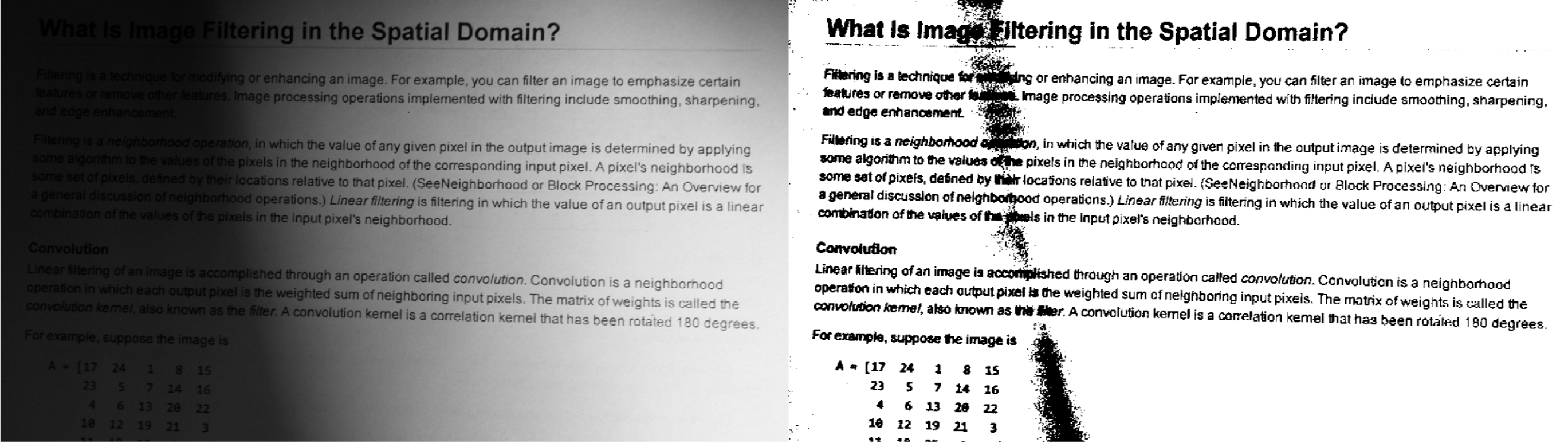
이미지의 이진화(Binarization) - adaptive thresholding

 

편향된 contrast를 갖는 이미지

 

 

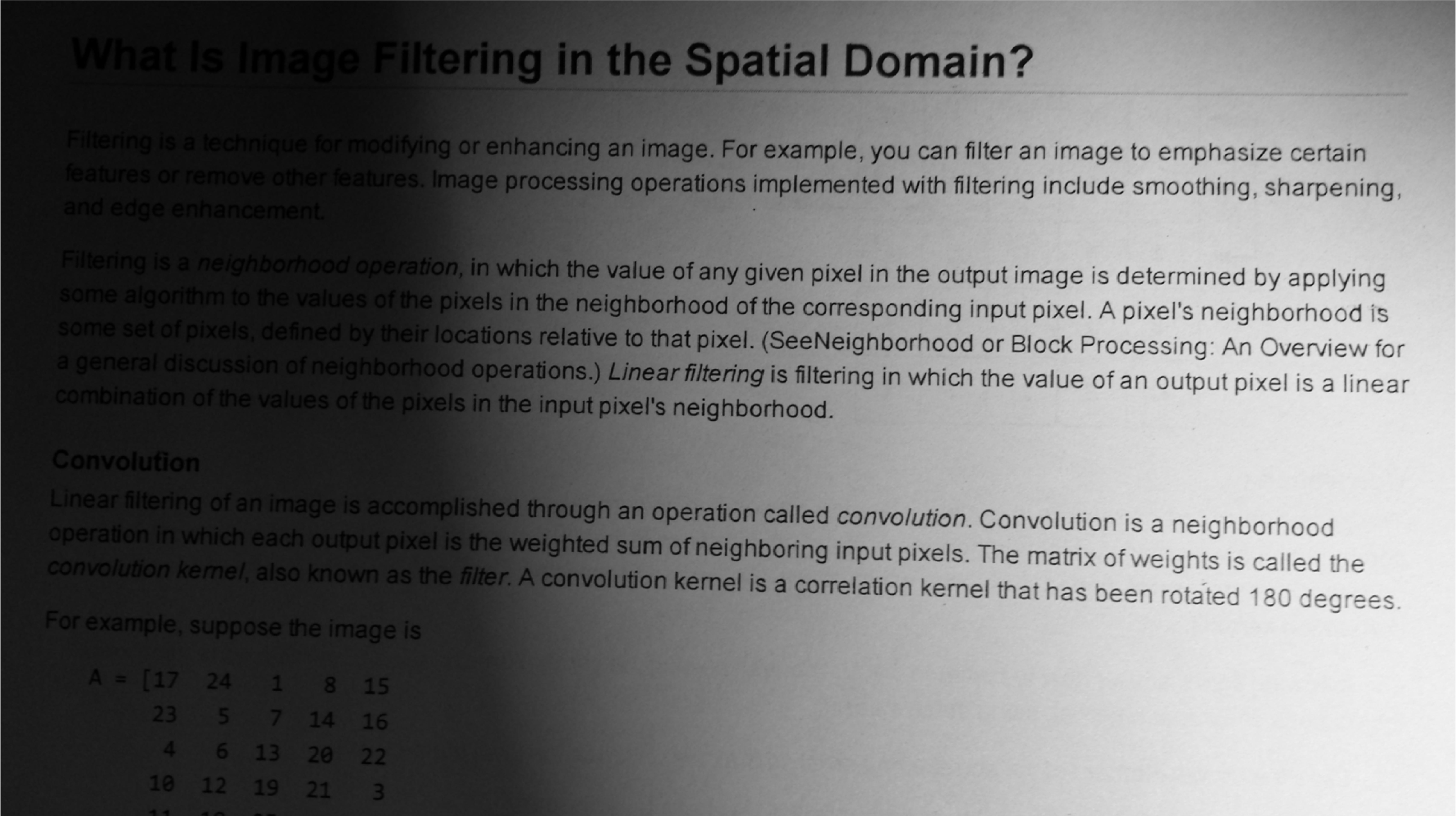
위의 이미지는 조명에 의해 편향된 contrast를 갖습니다. 앞서 본 global thresholding 의 관점에서 

본다면, 이미지의 binarization을 위한 threshold를 정하기 위해 위의 이미지 왼편의 어두운 영역과

오른편의 밝은 영역 사이 어디쯤엔가 균형을 맞춰야 할것이며 이는 수많은 시행착오를 필요로

할 것입니다.

( 위 이미지는 MATLAB의 built-in 이미지 이므로 따로 출처 표시를 하지 않았습니다. )

 

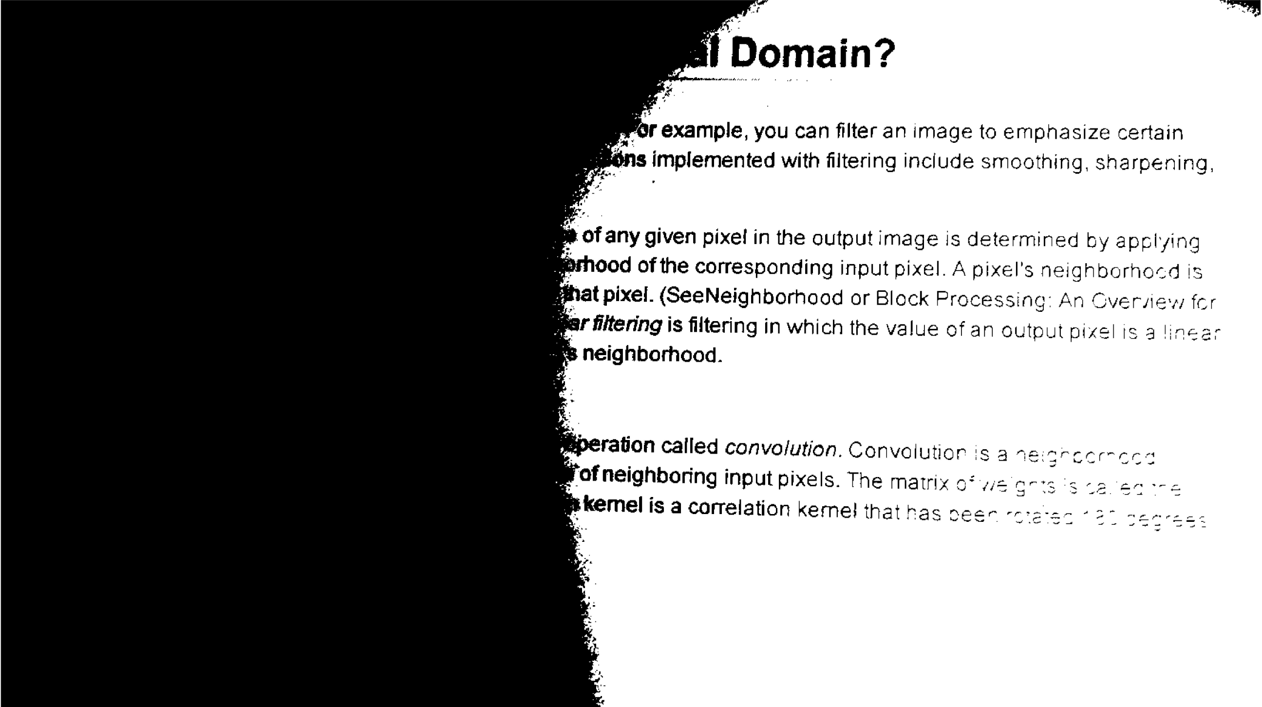
다음은 위 이미지에 Otsu algorithm을 적용한 global thresholding 결과 입니다.

이때 적용된 threshold 값은 110 입니다. 

 

 

편향된 contrast를 갖는 이미지에 Otsu algorithm을 적용한 결과 이미지

 

 

img2 = imread('printedtext.png');                      % the target image is built-in image in MATLAB
figure; imshow(img2)
figure; imhist(img2)

img_bw3 = imbinarize(img2);
figure, montage({img2,img_bw3})

% graythresh(img2) * 255

 

 

 

이처럼 균일하지 않은 조명을 갖거나 구역마다 contrast가 변동하는 이미지의 binarization 변환은

adaptive thresholding 방식을 선택하며, 이는 앞서 언급된 imbinarize( ) 함수의 입력 파라메터 지정을

통해 적용할 수 있습니다.

 

대상 이미지를 일정한 크기(또는 사용자가 지정한 크기)의 tile로써 구분하고, 각 tile에 속한 픽셀들의

평균값 - 또는 median(중간값), gaussian weighted mean(가우시안 가중 평균값)을 사용 할 수도 있음 -

을 threshold로써 각 tile 마다 binarization을 수행 하는것이 adaptive thresholding 입니다.

 

예를들어, 입력 이미지의 좌측 상단 부분을 하나의 tile로써 지정하여, 이 tile에 속한 픽셀들의 평균값을 

threshold로써 binarization을 수행하겠습니다. 이 tile의 크기는 입력 이미지 크기의 1/8에 해당하며 

평균값은 0-1 범위를 갖도록 정규화(normalization) 합니다.

 

 

이미지의 왼쪽 상단 tile에(좌측 이미지에 흰색 dash 상자) adaptive thresholding을 적용한 결과 (우측) 이미지

 

 

% tile size: approximately 1/8th of the size of the image
tile_size = 2*floor(size(img2)/16)+1;                % tile_size: [y-axis, x-axis]
img_tile = img2(1:tile_size(1),1:tile_size(2));      % a tile in the top left corner  

mean_img_tile = mean(img_tile(:));                 
img_tile_bw = imbinarize(img_tile, mean_img_tile/255);
figure; imshow(img2)
figure; imshow(img_tile_bw)

 

 

 

입력 이미지의 전경(foreground)은 전반적으로 배경(background) 보다 어둡습니다. 

이것을 adaptive thresholding에 하나의 입력 파라메터로써 추가하여 다음과 같은 binarization

결과를 얻었습니다.

 

 

편향된 contrast를 갖는 이미지에 adaptive thresholding을 적용한 결과 이미지

 

 

% search documentation of 'imbinarize' & 'adaptthresh' in HELP
img_bw4 = imbinarize(img2,'adaptive','ForegroundPolarity','dark');
figure; montage({img2, img_bw4})

 

 

 

 

 

 

마지막으로 본 글에 쓰인 모든 MATLAB 코드는 밑에 표시해 두었습니다.

 

img = imread('NCI-jdfn7Z03Qa4.jpg');

% gray scale conversion
img_gray = rgb2gray(img);
figure;
subplot(1, 2, 1); imshow(img); title('Original');
subplot(1, 2, 2); imshow(img_gray); title('Gray image');

% min-max-median 
min(img_gray(:))              % select all element. img_gray(:)
max(img_gray(:))
median(img_gray(:))

% histogram
figure;
imhist(img_gray);

% binarization
img_bw = imbinarize(img_gray);               % default method: Otsu algorithm
level = graythresh(img_gray) * 255           % level is a threshold Otsu algorithm operated
img_bw2 = imbinarize(img_gray, 100/255);     % giving a specified threshold 

figure;
subplot(1, 2, 1); imshow(img_bw); title('Not specified threshold value');
subplot(1, 2, 2); imshow(img_bw2); title('Specified threshold value');

% binarization - global thresholding
img = imread('NCI-jdfn7Z03Qa4.jpg');
img_gray = rgb2gray(img);                          % gray scale conversion
figure; imshow(img_gray)
figure; imhist(img_gray)

img_bw = imbinarize(img_gray, 100/255);            % giving a normalized threshold value
figure; montage({img_gray, img_bw})

img_bw2 = imbinarize(img_gray);                    % default method: Otsu algorithm
level = graythresh(img_gray) * 255                 % level is a global threshold value
figure; montage({img_gray, img_bw2})

% binarization - adaptive thresholding 
img2 = imread('printedtext.png');                  % the target image is built-in image in MATLAB
figure; imshow(img2)
figure; imhist(img2)

img_bw3 = imbinarize(img2);
figure, montage({img2,img_bw3})

% tile size: approximately 1/8th of the size of the image
tile_size = 2*floor(size(img2)/16)+1;              % tile_size: [y-axis, x-axis]
img_tile = img2(1:tile_size(1),1:tile_size(2));    % a tile in the top left corner  

mean_img_tile = mean(img_tile(:));                 
img_tile_bw = imbinarize(img_tile, mean_img_tile/255);
figure; imshow(img2)
figure; imshow(img_tile_bw)

% search documentation of 'imbinarize' & 'adaptthresh' in HELP
img_bw4 = imbinarize(img2,'adaptive','ForegroundPolarity','dark');
figure; montage({img2, img_bw4})

 

 

 

 

 

출처1: https://www.mathworks.com/help/matlab/ref/matlab.graphics.primitive.image-properties.html

Image appearance and behavior - MATLAB

 

 

출처2: https://unsplash.com/photos/jdfn7Z03Qa4

Published on September 7, 2021.6  Free to use under the Unsplash License

사진 작가: National Cancer Institute, Unsplash

 

 

출처3: https://www.mathworks.com/help/matlab/ref/rgb2gray.html

Convert RGB image or colormap to grayscale - MATLAB rgb2gray