[MATLAB 영상처리 기초 5] 이미지의 화질개선 - Normalization, Standardization
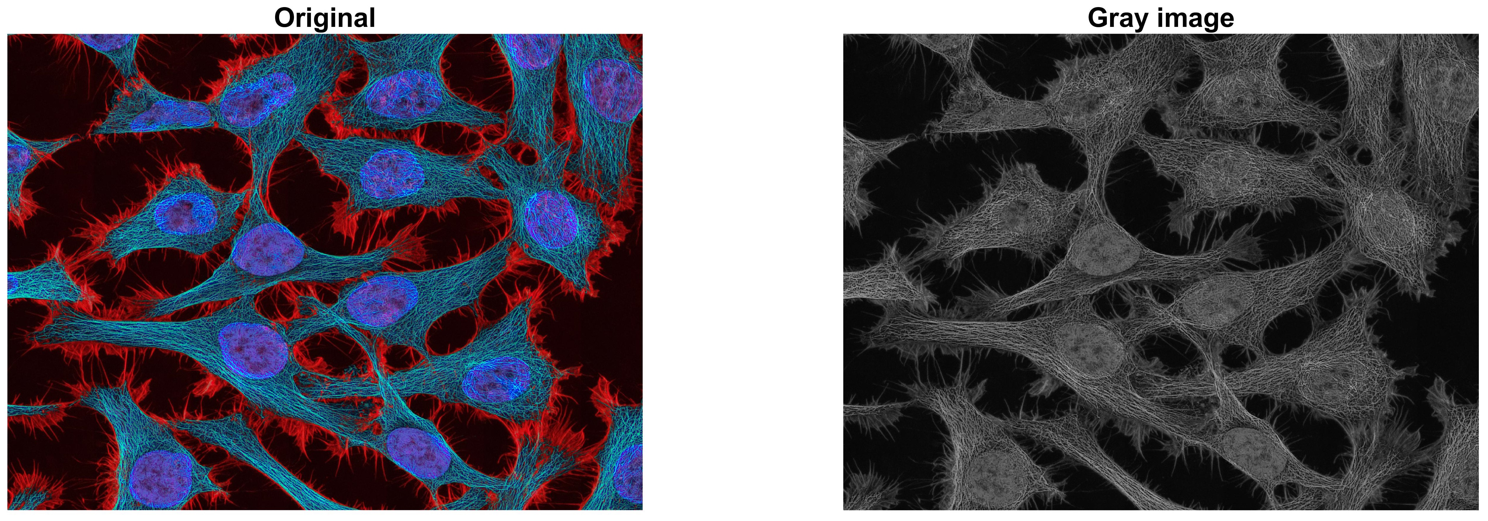
앞의 글 [MATLAB 영상처리 기초 3] 이미지의 픽셀값 다루기 - RGB2Gray 에서 RGB 컬러채널을 갖는
이미지의 grayscale 변환을 수행하였습니다.
그리고 grayscale 변환된 이미지 데이터는 MATLAB에서 기본적으로 uint8 형식을 가짐을 알 수 있었습니다.
Normalization
보통 MATLAB에서 Image Processing은 double 형식의 이미지 데이터를 다룹니다.
만일 정수형의 픽셀값을 대상으로 사칙연산(곱셈, 나눗셈 등)을 한다면, 연산후 소수점 이하의 값은
제거된다거나 표현가능 범위(여기서 uint8는 0 부터 255까지) 를 넘어서는 경우등 연산결과가
이미지상에 제대로 표현할 수 없기 때문입니다.
double등의 소수점 형식의 이미지 데이터는 최소 0부터 최대 1.0 까지 값의 범위를 갖도록 정규화 하는것이
일반적 입니다. uint8로부터의 변환 방법은, 간단하게도, 각 픽셀값을 (표현가능 범위)최대값인 255로
나누는 것입니다. 또는 MATLAB에서 제공하는 im2double( ) 명령어를 이용하는 것입니다.
( 위 이미지는 본 블로그 맨밑 출처 1에 가셔서 다운로드 받을 수 있습니다. )
img = imread('filename');
img_gray = rgb2gray(img);          % convert from RGB to grayscale image data
img_gray = im2double(img_gray);    % convert from uint8 to double type data
위의 작업을 통해 이미지 데이터 "img_gray" 는 픽셀값의 형식만이 변환된 것이므로 픽셀값의 분포는
변하지 않았을 것입니다. 그리고 앞의 글 [MATLAB 영상처리 기초 3] 이미지의 픽셀값 다루기 - Histogram
에 표시된 histogram에서 보듯이 대상 이미지의 grayscale (uint8 형식) 최소값은 0 이 아니고 최대값
또한 255가 아니였습니다.
만일 이미지 데이터의 최소, 최대값을 알고 있다면 이를 이용해 픽셀값의 분포범위를 0 - 1.0 으로써
rescaling이 - 픽셀의 최소값이 0, 최대값이 1.0으로써 rescaling을 뜻함 - 가능하며 픽셀값 분포가 넓게
퍼짐으로써 이미지 품질개선의 효과를 가질 수 있습니다.
( 이미지의 Contrast, Brightness, Gamma 조정은 [MATLAB 영상처리 기초 7] 참조 )
본 글에서는 간단하면서도 널리 사용되는 Min-Max Normalization을 수행해 보겠습니다.
Min-Max Normalization의 방법은 대상 이미지의 픽셀값을 최소값으로 뺀후 최대, 최소값 차이로 나눕니다.
min-max scaling = (X - Xmin) / (Xmax - Xmin)
(여기서 X: 픽셀값, Xmax: 픽셀의 최대값, Xmin: 픽셀의 최소값)
주의할점은 각 픽셀별로 연산해야 하므로 element-wise 나눗셈을 수행해야 합니다.
max_value = max(img_gray(:));
min_value = min(img_gray(:));

% pixel normalization: Scales values of the pixels in 0-1 range.
% min-max scaling = (X - Xmin) / (Xmax - Xmin)
img_gray_normal = (img_gray-min_value) ./ (max_value-min_value);

figure;
subplot(1,2,1); imshow(img_gray); title('Original image');
subplot(1,2,2); imshow(img_gray_normal); title('Rescaled image');

figure;
subplot(1,2,1); imhist(img_gray); title('Original image');
subplot(1,2,2); imhist(img_gray_normal); title('Rescaled image');
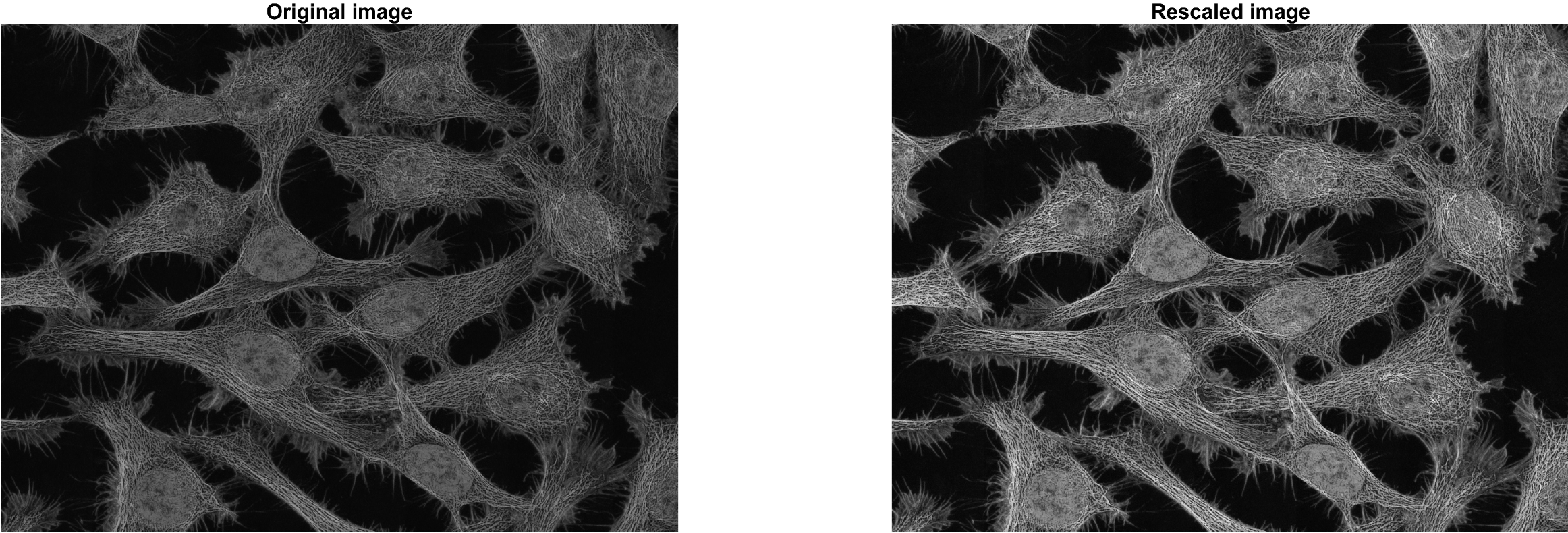
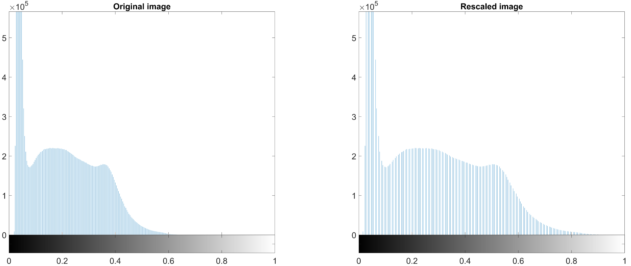
위 결과이미지 우측의 Rescale된 이미지는 좀 더 밝게 표현되며, 그 밑의 histogram은 그 이유를
잘 보여주고 있습니다. 좌측 대상 이미지의 histogram에서 알 수 있듯이, 픽셀값의 분포는
대략 0에서 0.4에 이르는 낮은 픽셀값 좁은 영역의 데이터분포를 갖지만 우측의 histogram은 0 - 0.8의
상대적으로 넓은 영역에 분포되어 있으므로 normalization된 이미지는 상대적으로 밝으며 좀 더 상세한
부분까지 표현가능한 것입니다.
이와같이 대상 이미지 데이터가 좁은영역에 픽셀값이 분포한 경우 normalization은 이미지 품질 개선의
효과를 보여줍니다.
Standardization
앞의 normalization과 병행되는 또다른 이미지 품질 개선 테크닉을 소개합니다.
대상 이미지의 픽셀값 분포가 넓은 영역에 고르지 않고 어둡거나 밝은 영역에 편향적으로 분포되어
있다면 - 예를들어 histogram에서 어두운 영역에 급격한 높은 봉우리를 갖고 밝은영역에 긴 꼬리를
갖을경우 - standardization이 큰 도움이 될것입니다.
이것은 픽셀값의 분포를 평균(mean) 0, 표준편차(standard deviation) 1 을 갖도록 scale시켜 줍니다.
즉, 픽셀값 분포의 대부분은 "0" 을 중심으로 위치함으로써 분포를 평탄하게 해줍니다.
Standardization은 픽셀값에서 픽셀의 평균값을 뺀후 픽셀의 표준편차로 나누어 구합니다.
standardization = (X - Xmean) / Xstd, 여기서 X: 픽셀값, Xmean: 픽셀의 평균, Xstd: 픽셀의 표준편차
주의할점은 각 픽셀별로 연산해야 하므로 element-wise 나눗셈을 수행해야 합니다.
% pixel Standardization– Scales values of the pixels to have
%                        0 mean and unit (1) variance.

% standardization = (X - Xmean) / Xstd
mean_value = mean(img_gray(:));
std_value = std(img_gray(:));
img_gray_stand = (img_gray-mean_value) ./ std_value;

figure;
subplot(1,2,1); imshow(imbinarize(img_gray)); title('Binary image of origin');
subplot(1,2,2); imshow(img_gray_stand); title('Standardized image');

[bin_cnt,~] = imhist(img_gray_stand);
figure; h = histogram(img_gray_stand,bin_cnt(1));
title('Histogram of standardized image');
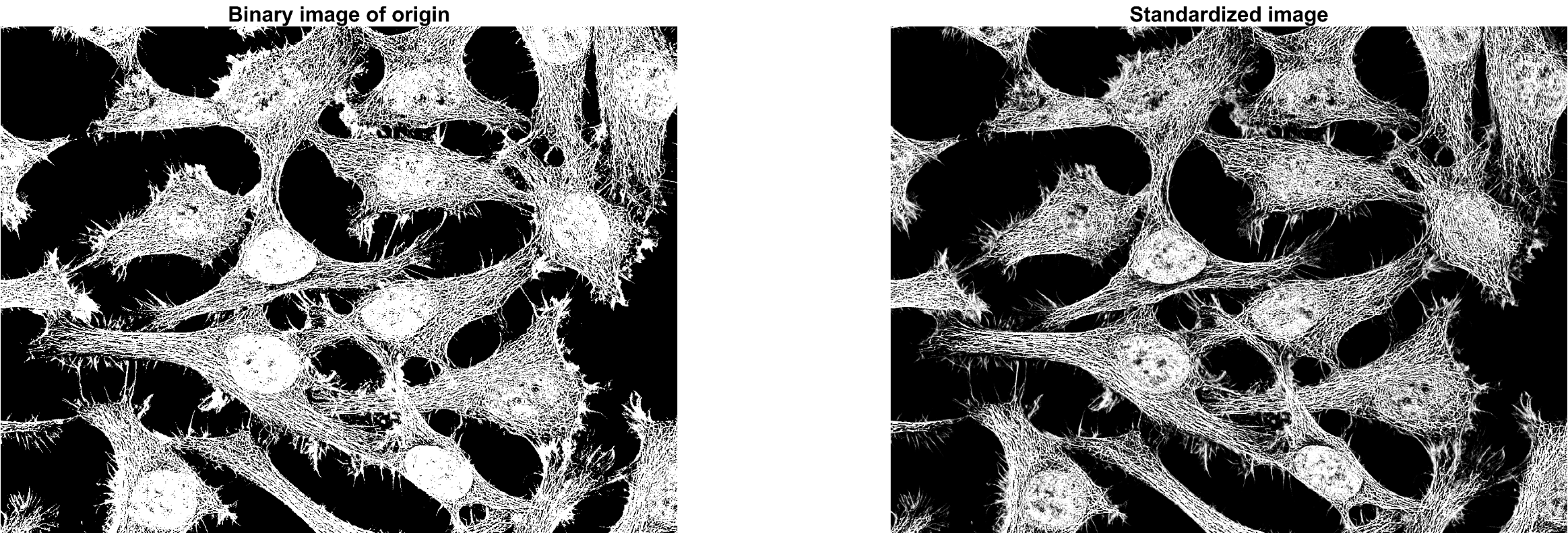

위의 결과 이미지 중 우측 이미지는 standardization을 수행한 결과로써 좌측의 Otsu 알고리즘을
이용한 Binarization 결과와 유사하게 보입니다. 그러나 우측의 standardization 결과 이미지를
자세히 본다면 cell(세포) 내, 외부의 미세한 형태적 특징을 좌측의 binarization 결과 보다 조금
더 자세히 볼 수 있습니다.
대상 이미지에 여러 cell(세포)들이 혼재한 경우 특정 cell(세포)을 추출 혹은 필터 마스크를
수행할 시, 개인적으로 미세한 형태적 특징을 고려해 binarization 보다는 standardization을
선호 합니다.
앞서 본 이미지의 normalization(정규화), standardization(표준화)는 deep learning에서 대규모
image-set 을 동일한 intensity 범위, scale로써 연산할 때 이용되는 테크닉입니다.
마지막으로 본 글에 쓰인 모든 MATLAB 코드는 밑에 표시해 두었습니다.
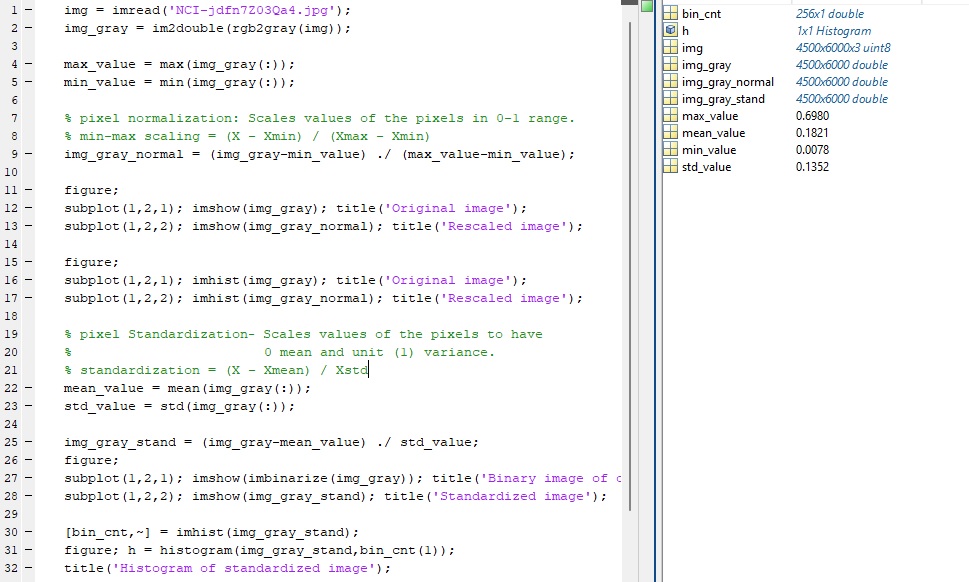
img = imread('NCI-jdfn7Z03Qa4.jpg');
img_gray = im2double(rgb2gray(img));

max_value = max(img_gray(:));
min_value = min(img_gray(:));

% pixel normalization: Scales values of the pixels in 0-1 range.
% min-max scaling = (X - Xmin) / (Xmax - Xmin)
img_gray_normal = (img_gray-min_value) ./ (max_value-min_value);

figure;
subplot(1,2,1); imshow(img_gray); title('Original image');
subplot(1,2,2); imshow(img_gray_normal); title('Rescaled image');

figure;
subplot(1,2,1); imhist(img_gray); title('Original image');
subplot(1,2,2); imhist(img_gray_normal); title('Rescaled image');

% pixel Standardization– Scales values of the pixels to have
%                        0 mean and unit (1) variance.

% standardization = (X - Xmean) / Xstd
mean_value = mean(img_gray(:));
std_value = std(img_gray(:));
img_gray_stand = (img_gray-mean_value) ./ std_value;

figure;
subplot(1,2,1); imshow(imbinarize(img_gray)); title('Binary image of origin');
subplot(1,2,2); imshow(img_gray_stand); title('Standardized image');

[bin_cnt,~] = imhist(img_gray_stand);
figure; h = histogram(img_gray_stand,bin_cnt(1));
title('Histogram of standardized image');
출처1: https://unsplash.com/photos/jdfn7Z03Qa4
Published on September 7, 2021.6 Free to use under the Unsplash License
사진 작가: National Cancer Institute, Unsplash
Cells from cervical cancer – Splash에서 National Cancer Institute의 이 사진 다운로드
unsplash.com